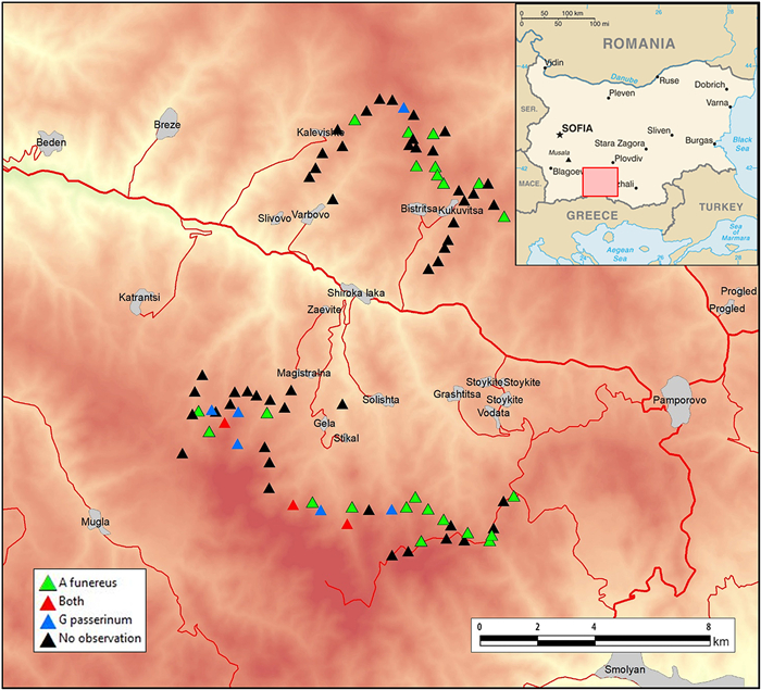
Figure
1.
Study area map.
| Citation: |
Boris P. Nikolov, Tzvetan Zlatanov, Thomas Groen, Stoyan Stoyanov, Iva Hristova-Nikolova, Manfred J. Lexer. 2022: Habitat requirements of Boreal Owl (Aegolius funereus) and Pygmy Owl (Glaucidium passerinum) in rear edge montane populations on the Balkan Peninsula. Avian Research, 13(1): 100020. DOI: 10.1016/j.avrs.2022.100020

|
Rear-edge populations of montane species are known to be vulnerable to environmental change, which could affect them by habitat reduction and isolation. Habitat requirements of two cold-adapted boreo-alpine owl species — Boreal Owl (Aegolius funereus) and Pygmy Owl (Glaucidium passerinum) — have been studied in refugial montane populations in the western Rhodopes, South Bulgaria. Data on owl presence and forest stand attributes recorded in situ have been used to identify significant predictors for owl occurrence. The results revealed Boreal Owl's preference for comparatively dense forests (high canopy closure values), big trees (diameter at breast height ≥50 cm) and large amount of fallen dead wood in penultimate stage of decay. For Pygmy Owl the only significant explanatory variable was the total amount of fallen dead wood. Results suggest preference of both owl species for forests with structural elements typical of old-growth forests (i.e., veteran trees, deadwood), the Pygmy Owl being less prone to inhabit managed forests. Being at the rear edge of their Palearctic breeding range in Europe both Boreal and Pygmy Owls are of high conservation value on the Balkan Peninsula. Hence, additional efforts are needed for their conservation in the light of climate change and resulting alteration of forest structural parameters. Current findings can be used for adjusting forest management practices in order to ensure both, sustainable profit from timber and continuous species survival.
It is widely accepted that climate change disproportionately threatens montane species — by reducing available habitat and by isolating their populations, the rear-edge populations being particularly affected by these pressures (Habibzadeh et al., 2021). Refining our understanding of rear-edge populations is considered essential to advance our ability to monitor, predict and plan for the impacts of environmental change on species range dynamics (Vilà-Cabrera et al., 2019).
The Balkan Peninsula holds some of the European relic montane populations of Boreal Owl (Aegolius funereus) and Pygmy Owl (Glaucidium passerinum) which are at the southernmost edge of their distribution ranges. Unlike the taiga zone and locally Central Europe where both species are intensively studied, little is known about their habitat requirements in these apparently isolated southern refugia (Mikkola, 1983; del Hoyo et al., 1999). Boreal and Pygmy Owls are cold-adapted boreo-alpine species which are expected to decline strongly or even disappear locally with climate change by the late 21st century on the southern edge of their Palearctic breeding range (Huntley et al., 2007; Brambilla et al., 2015), similar to many other Holarctic bird populations (Scridel et al., 2018). Both species face long-term decline in the boreal forests of northern Europe which is mainly attributable to the loss of mature and old-growth forests offering refuges against larger predators and better availability of main and alternative prey; in addition, the decline of Pygmy Owl population in this region was probably also fostered by climate change driven deteriorating population size of small mammals during the food-storing season due to increased rainfall (Korpimäki, 2021). A general population increase has been recently noted in both species in Central and South Europe but it has largely been explained by an increased survey effort during the last decades (Lehikoinen, 2020a, Lehikoinen, 2020b).
Both Boreal and Pygmy Owls are secondary cavity nesters and occupy territories of several hundred hectares, depending on key habitat parameters such as presence of old trees and/or standing and fallen deadwood providing hollows for nesting and suitable conditions for their prey, mostly small birds and mammals (von Blotzheim, 1980; Mikkola, 1983; Strøm and Sonerud, 2001). In Bulgaria, Boreal and Pygmy Owls are found mostly in the high mountains in the western part of the country, the Pygmy Owl being much rarer — about 100 pairs vs. 1025–1400 pairs (Shurulinkov et al., 2015; Spiridonov et al., 2015). Both species are of high conservation concern — on an international (Annex I of the EU Birds Directive) and national scale (Annex 2 of the Bulgarian Biodiversity Act, they are also listed in the Red Data Book of Bulgaria) (Shurulinkov et al., 2015; Spiridonov et al., 2015).
Boreal and many mountain forests face a considerable decrease of their structural and compositional heterogeneity as a result of historic and recent forest management activities, the amount of deadwood and snags and the maintenance of old-growth stand structures being critical for the conservation of biodiversity (Arnett et al., 2010; Bouget et al., 2014). In Bulgaria in particular, the total annual volume of roundwood harvested has been steadily increasing for the last two decades (GFSAF, 2000–2014). Additionally, during the period 2006–2013 the annual volume of illegal logging reached 2.5 million cubic meters or 25% of the total annual increment (WWF-Bulgaria, 2014). There is a concern that due to lack of knowledge and perceived lack of viable management alternatives the forest sector will not take the necessary steps to comprehensively assess the vulnerability, risks and uncertainties related to increases in harvest intensity (Zlatanov et al., 2017). These concerns are increased by an insufficient understanding of potential trade-offs and co-benefits between wood production and biodiversity conservation. Hence, it is of crucial importance to assess the occurrence of Boreal and Pygmy Owls in relation to various forest structural parameters and related forest management practices.
The overall aim of this study was to search for correlations between various forest parameters and presence of Boreal and Pygmy Owls. In particular, we aimed to identify the most important forest parameters influencing the occurrence of these two owl species.
The study was conducted in the western Rhodopes, within Shiroka Laka Forestry Enterprise totaling 9283.4 ha (97% of which are forests) (Fig. 1). The area is almost equally split in two parts by the valley of Shirokolashka River — northern (Chernatitsa ridge) and southern (Mursalitsa ridge), where the main mountain ridges are East-West oriented. The northern part of the area comprises of south-facing slopes reaching 1800–1900 m in altitude, while the southern part includes north-facing slopes of the highest part of the mountains, the massif of Perelik Peak (2191 m a.s.l.). Average annual precipitation at Shiroka Laka station (1050 m a.s.l.) is 850 mm, with precipitation being evenly distributed through most of the year. The driest period is August–October, with cumulative precipitation sums of 165 mm. The mean annual temperature at the station is 6 ℃, with a July mean temperature of 15.5 ℃ and a January mean temperature of minus 3 ℃ (Galabov, 1973). The area falls within Continental-Mediterranean climatic zone (Stanev et al., 1991).
Forests in the studied area are mainly Spruce (Picea abies) dominated, partly mixed with Scots Pine (Pinus sylvestris). Due to many societal and socio-economic changes during the last century, it is difficult to provide a unified definition of historic and recent forest management. Prior to the beginning of the 19th century, the area was subjected to heavy grazing, mainly by sheep. During the 1950s the forests were nationalized and the area partially depopulated. Stock breeding gradually lost its significance in the local economy. Silvicultural systems used were clearcutting and classical shelterwood, with rotation periods of around 120 years and annual allowable harvests less than or close to the annual increment of the forests (SLFEMP, 2007). During the post socialistic period (since 1990s), the forests in the study area were again privatized. Annual allowable harvest has increased since privatization, and now it often exceeds the annual increment of the forests.
Field sampling activities took place in September–October 2012, during the autumnal peak in the vocal activity of Boreal and Pygmy Owls (Kloubec and Pačenovsky, 1996; Pačenovsky and Shurulinkov, 2008; Korpimäki and Hakkarainen, 2012). Both species are considered resident and the autumn provides better access and milder weather in recording the territories of the potential breeding pairs in the study area (Pačenovsky and Shurulinkov, 2008). No post-natal and breeding dispersal is known so far for both species in Bulgaria (Shurulinkov et al., 2015; Spiridonov et al., 2015). In addition, there is no regular, multiannual cycle in the population size of rodents in South Europe, in contrast to northern Fennoscandia and the rest of northern Europe (Hanski et al., 1991), which is among the main drivers for dispersal and migratory movements in these two species in those regions (Mikkola, 1983). Of course, dispersal movements cannot be excluded, and the findings presumably show both territorial and some dispersing birds.
Eleven transects totaling 49.9 km (mean 4.5 km, SD = 1.78) were set above 1450 m a.s.l. (lowest point 1457 m, highest point 1974 m) along dirt roads within the coniferous belts of both main ridges — Chernatitsa and Mursalitsa, where both species have been previously recorded in several localities (Shurulinkov et al., 2007, 2015; Spiridonov et al., 2015). Nearly 65% of the total transect length (32.3 km) were set in Mursalitsa (Perelik massif), and the remainder (17.6 km) in Chernatitsa. A total of 85 predefined point counts were set, usually every 500–800 m (mean 668 m, n = 79) depending on the local topographic features and previous knowledge on the territory size in both species in Central and South Europe (Pačenovsky and Shurulinkov, 2008; Rajković et al., 2013). Owls were recorded at 34 of the points (40%) — one or both species per point. Special attention was paid to avoid possible double detection — where possible, the predefined point counts were set in separate secondary river valleys (so that the terrain was blocking the researcher's playback calls from spreading away too far), calling birds from already covered neighbouring point counts were not counted again, presence of two or more calling birds per one point count was considered only if they were detected at the same time.
The field protocol consisted of 2-min silent listening followed by a 10-min period of alternating imitations (both owl species territorial vocalisations) and silent listening. The imitations of Pygmy Owl always preceded those of Boreal Owl — although rare, records of interspecific aggression between these two species have been documented (Mikkola, 1983; Korpimäki and Hakkarainen, 2012). All surveys were conducted under favourable weather conditions: wind speed < 12 km/h (Beaufort scale 2 or less), no rain and temperatures close to seasonal average (Takats et al., 2001). Two censuses were done in early September and late September/early October in order to maximize the probability of recording the territorial males. Field surveys took place within 2–3-h periods before sunrise and after sunset.
Recording of forest stand attributes was performed in fixed area sample plots. For this purpose, two perpendicular transects were installed at each of the 85 predefined point counts. Transects were oriented in north-south and east-west direction and crossed at the centre point. Twenty five circular plots with a diameter of 11.3 m (plot area 100 m2) were established along each transect pair starting from the transect crossing point. As such, a total of 2125 plots were established in the study area. This sampling approach considers habitat heterogeneity in forests and ensures that recorded forest attributes do represent the habitat conditions of the localized owls (Seymour et al., 2002; Smith et al., 2008). Such an approach is rarely undertaken as inventorying a set of habitat variables on the ground is cost-, effort- and time-consuming (Hagan and Meeham, 2002).
The distance between two adjacent plots in each transect was 30 m. The selection of stand attributes recorded in each plot was based on a review of the literature (Hayward et al., 1993). It included, inter alia, canopy closure, and diameter at breast height (DBH) as well as height of all trees and snags (standing deadwood). All pieces of fallen deadwood larger than 7 cm were measured for length, maximum and minimum diameter. For fallen logs crossing the plot border only parts inside a plot were measured. In addition, snags and fallen deadwood were assigned to one of the five decay classes: (1) dead tree with no visual decay; (2) decay of the bark and small branches; (3) surface decay of the stem and larger branches, interior decay started to appear; (4) most part of stem and larger branches subjected to interior decay; and (5) stems entirely subjected to interior decay and partially destroyed, larger branches fully decayed. Canopy closure was accessed by a spherical densitometer (Lemmon, 1956). The DBH of the trees were measured with a calliper and assigned to DBH categories of 4 cm width. Height of the trees and snags as well as their distance to the plot centre were measured using a Vertex IV. The volume of stems and snags was determined by volume tables for individual trees (Krastanov and Raykov, 2004). The volume of broken snags and fallen deadwood pieces was calculated assuming the shape of a truncated cone. As suggested by Mihov (2005), 1 cm taper was assumed per meter of height when assessing the mean diameter of the snags. Resulting variables and their acronyms are shown in Table 1.
| Acronym | Description |
| stock | Total growing stock of all trees with DBH ≥8 cm (m3/ha) |
| fell3 | Percent of sample plots with fellings ≤3 years old |
| fell4.10 | Percent of sample plots with fellings 4–10 years old |
| fell10 | Percent of sample plots with fellings ≥10 years old |
| canclo3 | Percent of sample plots with canopy closure ≤0.3 |
| canclo68 | Percent of sample plots with canopy closure 0.6–0.8 |
| mcc | Mean canopy closure |
| dbh38trha | Number of trees in the sample plots with DBH ≥38 cm (per ha) |
| dbh38perc | Percent of sample plots with trees having DBH ≥38 cm |
| dbh42trha | Number of trees in the sample plots with DBH ≥42 cm (per ha) |
| dbh42perc | Percent of sample plots with trees having DBH ≥42 cm |
| dbh50trha | Number of trees in the sample plots with DBH ≥50 cm (per ha) |
| dbh50perc | Percent of sample plots with trees having DBH ≥50 cm |
| dbh58trha | Number of trees in the sample plots with DBH ≥58 cm (per ha) |
| dbh58perc | Percent of sample plots with trees having DBH ≥58 cm |
| fdw1 | Fallen dead wood in decay stage 1 (m3/ha) |
| fdw2 | Fallen dead wood in decay stage 2 (m3/ha) |
| fdw3 | Fallen dead wood in decay stage 3 (m3/ha) |
| fdw1-3 | Fallen dead wood in decay stages 1, 2 and 3 combined (m3/ha) |
| fdw4 | Fallen dead wood in decay stage 4 (m3/ha) |
| fdw5 | Fallen dead wood in decay stage 5 (m3/ha) |
| fdw4-5 | Fallen dead wood in decay stages 4 and 5 combined (m3/ha) |
| fdwsum | Total amount of fallen dead wood (m3/ha) |
| sdws1 | Standing dead wood in decay stage 1 (m3/ha) |
| sdws2 | Standing dead wood in decay stage 2 (m3/ha) |
| sdws3 | Standing dead wood in decay stage 3 (m3/ha) |
| sdw1-3 | Standing dead wood in decay stages 1, 2 and 3 combined (m3/ha) |
| sdws4 | Standing dead wood in decay stage 4 (m3/ha) |
| sdws5 | Standing dead wood in decay stage 5 (m3/ha) |
| sdws4-5 | Standing dead wood in decay stages 4 and 5 combined (m3/ha) |
| sdwsum | Total amount of standing dead wood (m3/ha) |
| DBH, diameter at breast height. | |
 DownLoad:
CSV
DownLoad:
CSV
To establish relationships between forest attributes and the presence of owl species we fitted generalized linear models (GLM) to our data. We employed the logit link function assuming a binomial error distribution (R Core Team, 2019). All variables were included in stepwise fitting procedures, one that considers removing variables (i.e., backwards) which was the preferred method, and one that considers adding variables (i.e., forward) in case the backward procedure could not converge. Both procedures were implemented using the step function in the R base package. We considered the full model as the upper limit, and a model with only an intercept as the lower limit. The fitting procedure followed the principle of parsimony by searching for a model with as few explanatory variables as possible that is still adequate regarding explained variation and model fit. Akaike's information criterion (AIC) was used as a means for model selection. AIC deals with the trade-off between the goodness of fit of the model and the simplicity of the model (i.e., the number of predictor variables). To test for multicollinearity between the predictor variables we employed the Variance Inflation Factor (VIF) (Hocking, 1976). To avoid multicollinearity VIF had to be below ten. In a final step we refitted the models with those predictor variables whose coefficients in the model were significant at p ≤ 0.05.
The basic residual statistics for the model (leverage, studentized residuals and DFBeta values) were also calculated to detect data points for which the model fits poorly, or which exert an undue influence on the modelled relationship of forest attributes and owl presence (Field et al., 2012).
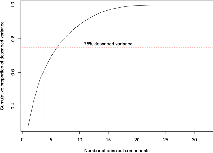
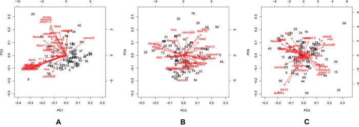
To gain a better understanding of the inner structure of our data a principal component analysis (PCA; Jolliffe, 2004) was performed. The PCA biplots were used to visualize how the significant predictor variables in the logistic regression models were related to the other forest attributes. We reviewed the first principal components that together explained at least 75% of the variation in the set of explanatory variables.
A total of 29 Boreal Owls in 27 territories and 10 Pygmy Owls in 9 territories were recorded: Boreal Owl — 10 birds/10 territories in Chernatitsa ridge, 19/17 in Mursalitsa; Pygmy Owl — just 1 bird (1 territory) in Chernatitsa, and 9 birds/8 territories in Mursalitsa. The relative density of Boreal Owls did not differ between Chernatitsa (0.57 territories/km transect line) and Mursalitsa (0.53 terr./km), while Pygmy Owls seemed better represented in Mursalitsa (0.25 terr./km) compared to Chernatitsa (0.06 terr./km).
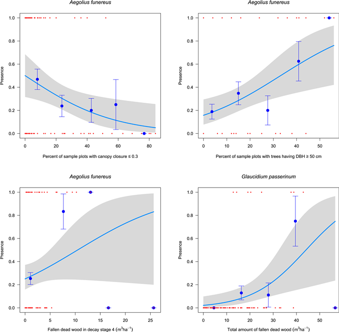
The stepwise backward fitting procedure found three variables that had a significant effect on the presence of Boreal Owl — percent of sample plots with canopy closure ≤0.3 (p < 0.01), percent of trees with diameter at breast height more than 50 cm (p < 0.01) and fallen dead wood in decay stage 4 (m3/ha) (p < 0.05). (Table 2A). We retained in the final model only the variables with statistically significant coefficients.
| Explanatory variables | B (SE) | 95% CI for odds ratio | |||
| A | Constant | −0.940 (0.583) | |||
| Percent of sample plots with canopy closure ≤0.3 | −0.042 (0.018)** | 0.922 | 0.959 | 0.990 | |
| Percent of sample plots with trees having DBH ≥50 cm | 0.038 (0.020)* | 1.000 | 1.039 | 1.083 | |
| Fallen dead wood stage of decay 4 | 0.175 (0.071)** | 1.040 | 1.191 | 1.387 | |
| Model χ2 (3) = 18.48, p < 0.001, AIC = 87.261, *p < 0.1, **p < 0.05. | |||||
| B | Constant | −3.812 (0.815)*** | |||
| Total amount of fallen dead wood | 0.087 (0.032)** | 1.029 | 1.090 | 1.168 | |
| Model χ2 (1) = 8.594, p < 0.01, AIC = 47.419, **p < 0.01, ***p < 0.001. | |||||
DownLoad:
CSV
No backward regression model could be established for Pygmy Owl. However, the stepwise forward procedure yielded a model with total amount of fallen dead wood as significant predictor (Table 2B). The basic residual statistics (leverage, studentized residuals and DFBeta values) indicated a good fit of both models to the observed data. All cases had DFBetas less than 1, and leverage statistics were very close to the calculated expected value of 0.05, which means that there were no influential cases having an effect on the model. The studentized residuals all had values of less than ±2.
The principal component analysis revealed that six principal components are needed to explain at least 75% of the variation in the set of explanatory variables (Fig. 2). There was strong clustering along the first two principal components (Fig. 3; panel A) with at least four very well distinguished clusters. Not surprisingly, there was a strong clustering of all DBH class variables (Fig. 3; panel A), so they essentially contain similar information. But from an ecological point of view, trees with a DBH ≥50 cm are expected to be more relevant for both owl species. The total amount of fallen dead wood represented one of the clusters (Fig. 3; panel A) and significantly influenced the presence of both owl species. Percent of sample plots with canopy closure ≤0.3 (Fig. 3; panel A) stands out as a variable that contains a lot of unique information. For the fallen deadwood indicators, fallen dead wood in decay stage 4 (m3/ha) was related most to the third principal component (Fig. 3; panel B). The fifth and sixth principal components didn't yield any further insights into the variables included in the models (Fig. 3; panel C). The PCA also revealed multicollinearity in the overall data set, however, the VIFs associated with the predictor variables included in both models were all below 10, indicating that multicollinearity in the final models was sufficiently controlled.
We performed a graphical test of the fit of the logistic models to the variables included in the GLM. We plotted the fitted logistic model through the (0, 1) scatterplot of the data for both species for each variable separately (Fig. 4). The data range was split into five even sectors and empirical probabilities with their standard errors were shown together with the 95% confidence intervals along each logistic model function. Evidently, the logistic model for Boreal Owl shows a good fit, particularly regarding canopy closure and percentage of trees having a DBH > 50 cm. However, it fits less well with the fallen deadwood in decay stage 4. The logistic model predicting the presence of Pygmy Owl showed a rather poor fit. This may be due to the relatively few presence points for this species.
Although data for Boreal and Pygmy Owl breeding density in Bulgaria and the Balkans in general are scarce, the results from the western Rhodopes allow some comparisons. During the present study Boreal Owl was found to occur at densities comparable with those in Pirin Mt. in southwestern Bulgaria (6.9 terr./10 km2), central Serbia −7.7 terr./10 km2 (24 km2 study area), Slovenia (2.8 terr./10 km2, 32 km2 study area), as well as elsewhere in Europe — from 0.3 to 6.9 terr./10 km2 depending on the size of the study area and prevailing habitats (Shurulinkov et al., 2003; Vrezec, 2003; see Rajković et al., 2013). In Eurasia fluctuations in breeding populations increase to the north and east, perhaps dependent not only on vole cycles but also on depth of annual snow cover (feeding inhibited by deep snow) (del Hoyo et al., 1999). In North America the Boreal Owl appears to be widely distributed but occurring at low densities — 0.15–3 terr./10 km2 (Lane et al., 2001). Pygmy Owl density in Mursalitsa was found to be rather similar to that previously recorded in the western Rhodopes — 2.18 terr./10 km2 (Shurulinkov et al., 2007). Pačenovsky and Shurulinkov (2008) report an average density of 3.9 terr./10 km2 in SW Bulgaria — twice as low as in the Western Carpathians, which is probably caused by the fact that we looked at their distribution at the edge of the range area of the species and the higher isolation level in the Balkans. Transect census in the same area (Rila Mt) revealed a Pygmy Owl density of 0.40–0.46 terr./km (Spiridonov et al., 2015). Some of the highest species densities have been recorded in Northern Europe — up to 30 pairs/10 km2; subjected to fluctuations (similarly to Boreal Owl, mainly due to weather conditions and rodent cycles), they vary locally over 100-fold; much less population fluctuations are known for the mountains in Central Europe (del Hoyo et al., 1999).
Although both species — Boreal Owl and Pygmy Owl — are not studied so extensively on the Balkans, compared to Northern or Central Europe, for example, it appears that their populations in these southernmost European refugia do not face big fluctuations. That is why modelling of their habitat requirements at these comparatively low densities would be beneficial both from conservation and species management point of view.
The statistical methods applied revealed three main explanatory variables for the presence of Boreal Owl — percent of sample plots with canopy closure ≤0.3, percent of sample plots with trees having DBH ≥50 cm and fallen dead wood stage of decay 4. Our findings of Boreal Owl's preference for comparatively dense forests (high canopy closure values) are well supported by published data (Korpimäki and Hakkarainen, 2012). In North America the species' summer roosts were in dense shaded forests with higher canopy cover and tree density (i.e., indicating cool microhabitats), compared to the winter roost sites. Boreal Owl is well adapted to severe winter climate conditions, but suffers physiological stress during summer due to high temperatures (Hayward et al., 1993). This may become even more relevant in a warmer climate.
The remaining two variables — big trees and large amount of dead wood — are among the vital parameters typical for old-growth forests. The high affinity of Boreal and especially of Pygmy Owls to mature forests (both as hunting and nesting habitat) is well-known (Mikkola, 1983; Strøm and Sonerud, 2001; Korpimäki and Hakkarainen, 2012). Laaksonen et al. (2004) showed that lifetime reproductive success of Boreal Owls increased with a higher proportion of old-growth coniferous forest in the territory, which underlines the importance of mature coniferous forests as the stronghold of the species. Both Boreal Owl and the Black Woodpecker (Dryocopus martius) have been reported as umbrella and/or keystone species and the occurrence of both of them can represent priority areas for the conservation of forest (Brambilla et al., 2013). Pygmy Owl has been found to be among the bird species which are the best multiscale indicators for high breeding bird assemblage diversity in boreal forests (Pakkala et al., 2014).
Both Boreal and Pygmy Owls are obligate secondary cavity nesters, breeding in cavities excavated by woodpeckers or holes created by fungal decay and insects (Mikkola, 1983; del Hoyo et al., 1999). In Eurasian coniferous forests, the Boreal Owl is mainly dependent on cavities excavated by Black Woodpecker (Korpimäki and Hakkarainen, 2012), whereas in North America, the Pileated Woodpecker (Dryocopus pileatus) and Common Flicker (Colaptes auratus) are the main cavity-suppliers for the species (Hayward and Hayward, 1993). This underlines the importance of presence of trees with sufficient girth allowing for cavities of appropriate dimensions.
The amount of fallen deadwood seems to be important for both owl species, as the only explanatory variable for Pygmy Owl was found to be the total amount of fallen dead wood, and a similar parameter was found to be important for Boreal Owl (amount of fallen dead wood in penultimate stage of decay). This is probably connected indirectly to prey availability — it has been shown that high volumes of late-decay coarse woody debris favours local diversity of small mammals (Fauteux et al., 2013).
Standing deadwood (snags) — in addition to the fallen deadwood — is also of virtual importance for maintaining forest biodiversity, and especially cavity-nesting bird species (Korpimäki and Hakkarainen, 2012; Barbaro et al., 2016). Since the late 1990s many studies on multiple-species interactions between snag-users and snags shifted the focus of snag management from a single-species to a multi-species perspective which has far-reaching implications for the maintenance of the complex ecological processes that are driven by snag dynamics (see Drapeau et al., 2009). Although our modelling results suggest that standing deadwood appears to be of no significant importance to Boreal Owl it is known from other studies that retaining standing (and fallen) wood on the site will mitigate the negative impacts of the logging activities over the long-term — maintaining both cavity and prey availability (Hayward, 1997).
Deadwood proved to be extremely important for the conservation of habitat for more than 25% of the mountain forest fauna and flora (see Humphrey et al., 2004) and for key ecological processes in forest ecosystems in general (see Drapeau et al., 2009). Hence measures of deadwood for consideration as potential indicators of saproxylic and epixylic diversity have been developed for different forest types within Europe, including boreal coniferous forests. Deadwood should be considered important not only as nest trees but also as key element in the food webs in the boreal forest, like it has been shown for woodpeckers (Drapeau et al., 2009).
There is strong evidence that some recent outbreaks of bark beetles and defoliating insects are influenced by climate change and are having a large impact on ecosystems (Pureswaran et al., 2018). One of the outcomes is the availability of bigger quantities of deadwood, which can prove beneficial for many species (Barbaro et al., 2016). A positive correlation between deadwood volume and the density of birds — both primary and secondary cavity nesters, was recently shown by Bujoczek et al. (2021).
Our data suggest that Boreal Owl seems to be more tolerant to habitats where logging activities have taken place in the past (more than 10 years), unlike Pygmy Owl. Both species often occupy old-growth forests or forests with patches of old-growth stands but can benefit from the edges with stands of younger successional stages or open spaces (von Blotzheim, 1980; Mikkola, 1983; Strøm and Sonerud, 2001). However, attention should be paid to the level of fragmentation which could have marked negative impacts on various species of conservation concern (Mikusiński et al., 2018).
In order to achieve and then to maintain favourable conservation status of both owl species adequate forest managing practices should be adopted. It is known that substantial knowledge on habitat requirements, as well as various behavioural aspects of the species is needed for estimating adequate and detailed forest management implications (Kouki et al., 2001). According to current Bulgarian forestry legislation, no clearcuts are allowed in mountain forests. The regeneration system frequently used in managed forests in the Rhodopes is the shelterwood system with regeneration periods of 20 years. In group selection systems the regeneration period usually takes 40 years or more, hence higher probability of achieving a greater diameter in standing trees. As such, group selection systems seem to be a valuable alternative to classical shelterwood systems. However, the increased illegal logging and "by-passing" the legal practices do not contribute to sustainable use of the timber resources and biodiversity conservation (WWF-Bulgaria, 2014).
In general, the retention of stands (at least 1% of the forest area) with 30–40 large (80–100 cm diameter), and old (over 100 years) trees per ha is recommended to enhance deadwood habitat in spruce plantations (Humphrey et al., 2004), as well as to increase habitat heterogeneity. A positive correlation between habitat heterogeneity/diversity and bird species diversity has been documented in a number of studies (see Tews et al., 2004).
Our results show that forest structure is important for both Boreal and Pygmy Owls. Hence management that aims at conserving these forest structures will be important for the maintenance of these two owl species at the edge of their European distribution range. One might expect that the potential impact of expected climatic change on these species will be exacerbated when also stand structure is not optimal. Then the combined effects of unsuitable habitat conditions and climate change might lead to an accelerated decline of the presence of these two owl species in the Balkan Peninsula.
Results suggest preference of both owl species for forests with elements typical of old-growth forests, the Pygmy Owl being less prone to inhabit managed forests. Being at the rear edge of their range in Europe both Boreal and Pygmy Owls are of high conservation value on the Balkan Peninsula and additional efforts are needed for their conservation in the light of climate change and resulting alteration of forest structural parameters. Current findings can be used for adjusting forest management practices in order to ensure both sustainable profit from timber and continuous species survival.
All authors designed the study. BN, TZ and IH-N performed the field studies. SS, TG, TZ and BN carried out the analyses. BN produced the first draft, and all authors contributed substantially to the final manuscript. All authors read and approved the final manuscript.
The authors declare that they have no competing interests.
All field activities were conducted within the project "Advanced multifunctional forest management in European mountain ranges" (ARANGE) funded by the Seventh Framework Programme of the European Union. A number of people helped us both with field and office work — our sincere thanks go to all of them: Georgi Gogushev, Georgi Hinkov, Ivaylo Velichkov, Georgi Georgiev, Magdalena Zlatanova, Hristina Hristova, Emil Komitov and Dimitar Angelov.
|
del Hoyo, J., Elliott, A., Sargatal, J., 1999. Handbook of the Birds of the World. Vol. 5: Barn-owls to Hummingbirds. Lynx Edicions, Barcelona.
|
|
Field, A.P., Miles, J., Field, Z., 2012. Discovering Statistics Using R. Sage, London.
|
|
Galabov, Z., 1973. Atlas of the People's Republic of Bulgaria. Main Bureau of Geodesy and Cartography, Sofia.
|
|
GFSAF, 2000-2014. Report Forms 5 GF (Forest Fund). Bulgarian State Forest Agency, Sofia.
|
|
Hagan, J.M., Meeham, A.L., 2002. The effectiveness of stand-level and landscape-level variables for explaining bird occurrence in an industrial forest. For. Sci. 48, 231-242.
|
|
Hayward, G.D., 1997. Forest management and conservation of Boreal Owls in North America. J. Raptor Res. 31, 114-124.
|
|
Hayward, G.D., Hayward, P.H., 1993. Boreal owl Aegolius funereus. In: Poole, A., Gill, F. (Eds. ), The Birds of North America. Academy of Natural Sciences and American Ornithologists Union, Philadelphia, pp. 1–19.
|
|
Hayward, G.D., Hayward, P.H., Garton, E.O., 1993. Ecology of Boreal Owls in the Northern Rocky Mountains, USA. Wildl. Monogr. 124, 1-59.
|
|
Humphrey, J.W., Sippola, A-L., Lemperiere, G., Dodelin, B., Alexander, K.N.A., Butler, J.E., 2004. Deadwood as an indicator of biodiversity in European forests: from theory to operational guidance. In: Marchetti, M., (Ed. ), Monitoring and Indicators of Forest Biodiversity in Europe - From Ideas to Operationality. EFI Proceedings, Saarijarvi, pp. 193-206.
|
|
Huntley, B., Green, R.E., Collingham, Y.C., Willis, S.G., 2007. A Climatic Atlas of European Breeding Birds. Lynx, Barcelona.
|
|
Jolliffe, I.T., 2004. Principal Component Analysis. 2nd ed. Springer, New York.
|
|
Kloubec, B., Pacenovsky, S., 1996. Vocal activity of Tengmalm's Owl (Aegolius funereus) in southern Bohemia and eastern Slovakia: circadian and seasonal course, effects on intensity. Buteo 8, 5-22.
|
|
Korpimaki, E., 2021. Habitat degradation and climate change as drivers of long-term declines of two forest-dwelling owl populations in boreal forest. Airo 29, 278-290.
|
|
Korpimaki, E., Hakkarainen, H., 2012. The Boreal Owl: Ecology, Behaviour, and Conservation of a Forest-Dwelling Predator. Cambridge Univ. Press, Cambridge.
|
|
Kouki, J., Lofman, S., Martikainen, P., Rouvinen, S., Uotila, A., 2001. Forest fragmentation in Fennoscandia: linking habitat requirements of wood-associated threatened species to landscape and habitat changes. Scand. J. For. Res. 3, 27-37.
|
|
Krastanov, K., Raykov, R., 2004. Dendrobiology Reference Book. BULPROFOR, Sofia.
|
|
Laaksonen, T., Hakkarainen, H., Korpimaki, E., 2004. Lifetime reproduction of a forestdwelling owl increases with age and area of forests. Proc. R. Soc. Lond. B. 271, S461-S464.
|
|
Lane, W.H., Andersen, D.E., Nicholls, T.H., 2001. Distribution, abundance, and habitat use of singing male Boreal Owls in Northeast Minnesota. J. Raptor Res. 35, 130-140.
|
|
Lehikoinen, A., 2020a. Eurasian Pygmy-owl Glaucidium passerinum. In: Keller, V., Herrando, S., Voříšek, P. (Eds. ), European Breeding Bird Atlas 2: Distribution, Abundance and Change. European Bird Census Council & Lynx Edicions, Barcelona, pp. 412–413.
|
|
Lehikoinen, A., 2020b. Boreal Owl Aegolius funereus. In: Keller, V., Herrando, S., Voříšek, P. (Eds. ), European Breeding Bird Atlas 2: Distribution, Abundance and Change. European Bird Census Council & Lynx Edicions, Barcelona, pp. 416–417.
|
|
Lemmon, P.E., 1956. A spherical densitometer for estimating forest overstory density. For. Sci. 2, 314-320.
|
|
Mihov, I., 2005. Forest mensuration. RIK Litera, Sofia. (In Bulgarian).
|
|
Mikkola, H., 1983. Owls of Europe. T & AD Poyser, London.
|
|
Shurulinkov, P., Stoyanov, G., Tzvetkov, P., Vulchev, K., Kolchagov, R., Ilieva, M., 2003. Distribution and abundance of Tengmalm's Owl Aegolius funereus on Mount Pirin, south-west Bulgaria. Sandgrouse 25, 103-109.
|
|
Shurulinkov, P., Ralev, A., Daskalova, G., Chakarov, N., 2007. Distribution, numbers and habitat of Pygmy Owl Glaucidium passerinum in Rhodopes Mts (S Bulgaria). Acrocephalus 28, 161-165.
|
|
Shurulinkov, P., Spiridonov, Z., Zlatanov, T., Nikolov, B., Nikolov, S., Stanchev, R., 2015. Boreal Owl (Aegolius funereus). In: Golemanski, V., et al., (Eds. ), Red Data Book of Bulgaria. Vol. 2. Animals. BAS & MOEW, Sofia, pp. 274.
|
|
Spiridonov, Z., Nikolov, B., Shurulinkov, P., 2015. Pygmy Owl (Glaucidium passerinum). In: Golemanski, V. (Ed. ), et al., Red Data Book of Bulgaria. Vol. 2. Animals. BAS & MOEW, Sofia, p. 191.
|
|
Stanev, S., Kyuchukova, M., Lingova, S., 1991. The climate of Bulgaria. BAS, Sofia. (In Bulgarian with English summary).
|
|
Stroem, H., Sonerud, G.A., 2001. Home range and habitat selection in the Pygmy Owl Glaucidium passerinum. Ornis Fennica 78, 145-158.
|
|
Takats, D.L., Francis, C.M., Holroyd, G.L., Duncan, J.R., Mazur, K.M., Cannings, R.J., et al., 2001. Guidelines for Nocturnal Owl Monitoring in North America. Beaverhill Bird Observatory and Bird Studies Canada, Edmonton.
|
|
von Blotzheim, U.N.G., 1980. Handbuch der Vogel Mitteleuropas. Akademische Verlagsgesellschaft, Frankfurt am Main.
|
|
Vrezec, A., 2003. Breeding density and altitudinal distribution of the Ural, tawny, and boreal owls in North Dinaric Alps (central Slovenia). J. Raptor Res. 37, 55-62.
|
Figures(4) / Tables(2)


| Acronym | Description |
| stock | Total growing stock of all trees with DBH ≥8 cm (m3/ha) |
| fell3 | Percent of sample plots with fellings ≤3 years old |
| fell4.10 | Percent of sample plots with fellings 4–10 years old |
| fell10 | Percent of sample plots with fellings ≥10 years old |
| canclo3 | Percent of sample plots with canopy closure ≤0.3 |
| canclo68 | Percent of sample plots with canopy closure 0.6–0.8 |
| mcc | Mean canopy closure |
| dbh38trha | Number of trees in the sample plots with DBH ≥38 cm (per ha) |
| dbh38perc | Percent of sample plots with trees having DBH ≥38 cm |
| dbh42trha | Number of trees in the sample plots with DBH ≥42 cm (per ha) |
| dbh42perc | Percent of sample plots with trees having DBH ≥42 cm |
| dbh50trha | Number of trees in the sample plots with DBH ≥50 cm (per ha) |
| dbh50perc | Percent of sample plots with trees having DBH ≥50 cm |
| dbh58trha | Number of trees in the sample plots with DBH ≥58 cm (per ha) |
| dbh58perc | Percent of sample plots with trees having DBH ≥58 cm |
| fdw1 | Fallen dead wood in decay stage 1 (m3/ha) |
| fdw2 | Fallen dead wood in decay stage 2 (m3/ha) |
| fdw3 | Fallen dead wood in decay stage 3 (m3/ha) |
| fdw1-3 | Fallen dead wood in decay stages 1, 2 and 3 combined (m3/ha) |
| fdw4 | Fallen dead wood in decay stage 4 (m3/ha) |
| fdw5 | Fallen dead wood in decay stage 5 (m3/ha) |
| fdw4-5 | Fallen dead wood in decay stages 4 and 5 combined (m3/ha) |
| fdwsum | Total amount of fallen dead wood (m3/ha) |
| sdws1 | Standing dead wood in decay stage 1 (m3/ha) |
| sdws2 | Standing dead wood in decay stage 2 (m3/ha) |
| sdws3 | Standing dead wood in decay stage 3 (m3/ha) |
| sdw1-3 | Standing dead wood in decay stages 1, 2 and 3 combined (m3/ha) |
| sdws4 | Standing dead wood in decay stage 4 (m3/ha) |
| sdws5 | Standing dead wood in decay stage 5 (m3/ha) |
| sdws4-5 | Standing dead wood in decay stages 4 and 5 combined (m3/ha) |
| sdwsum | Total amount of standing dead wood (m3/ha) |
| DBH, diameter at breast height. | |
DownLoad:
CSV
| Explanatory variables | B (SE) | 95% CI for odds ratio | |||
| A | Constant | −0.940 (0.583) | |||
| Percent of sample plots with canopy closure ≤0.3 | −0.042 (0.018)** | 0.922 | 0.959 | 0.990 | |
| Percent of sample plots with trees having DBH ≥50 cm | 0.038 (0.020)* | 1.000 | 1.039 | 1.083 | |
| Fallen dead wood stage of decay 4 | 0.175 (0.071)** | 1.040 | 1.191 | 1.387 | |
| Model χ2 (3) = 18.48, p < 0.001, AIC = 87.261, *p < 0.1, **p < 0.05. | |||||
| B | Constant | −3.812 (0.815)*** | |||
| Total amount of fallen dead wood | 0.087 (0.032)** | 1.029 | 1.090 | 1.168 | |
| Model χ2 (1) = 8.594, p < 0.01, AIC = 47.419, **p < 0.01, ***p < 0.001. | |||||
DownLoad:
CSV
 Email Alerts
 RSS Feeds