On the potential of documenting decadal-scale avifaunal change from before-and-after comparisons of museum and observational data across North America

1.   Introduction

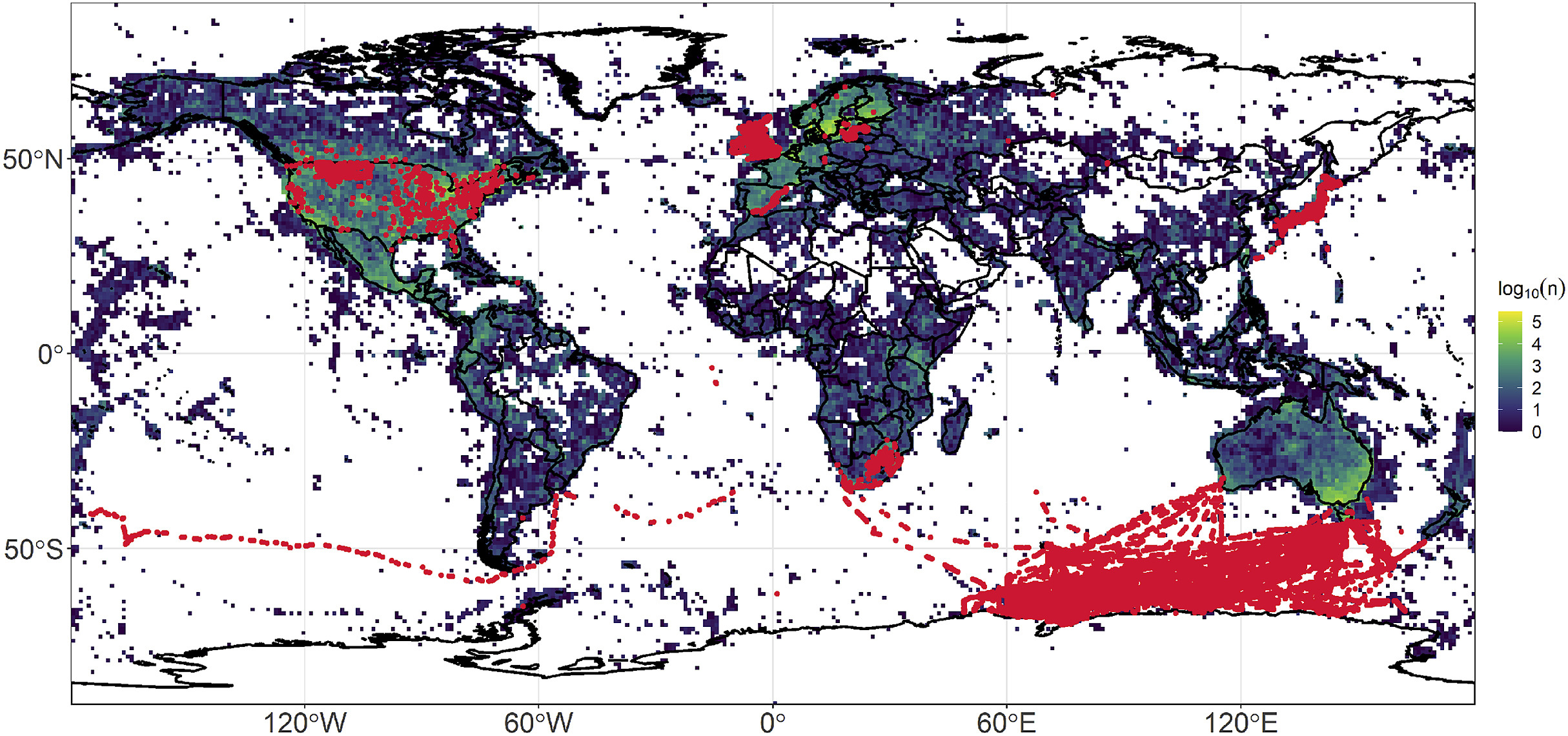
Biotic change and species turnover in local communities are of intense interest in organismal biology, with spatial and temporal changes in species composition occurring on multiple scales (Soininen, 2010). However, the time scales involved in studies to date have been rather disparate: systematics and paleontology work with these questions on coarse and deep time scales, extending back millions of years, and with a temporal resolution of thousands of years or more (e.g., Webb, 1991). On the other hand, ecology focuses on time scales that are far shorter, on the order of days to years (e.g., Levin, 1992). The decades-to-centuries time scale is quite difficult to fill, for lack of easily available datasets with which to assess questions associated with biotic change, although some studies have bridged the gap in time scales (e.g., Laurance et al., 2006; Tingley et al., 2009; Rosenberg et al., 2019). Among the few long-term time series studies available, the vast majority have been done in North America and Europe (e.g., Root, 1988a; Sauer et al., 2017b; Dornelas et al., 2018), and most European monitoring schemes started after the 1980s, having an average time span of 15 years (Mihoub et al., 2017). Therefore, knowledge on species turnover across the globe has several gaps in space and time, with available time series data concentrated in developed countries, and biodiversity-rich regions and hotspots lacking such information (Fig. 1).

Figure  1.  Global distribution of sites (red dots) from 41 time series studies on birds (BioTime database, ∼1.4 ​× ​10⁶ records, Dornelas et al., 2018). The raster image (1° resolution) represents the log number of unique bird records (species ​× ​date ​× ​site; ∼19 ​× ​10⁶ records) from the GBIF database before 1980.

DownLoad: Full-Size Img PowerPoint

Major advances in biodiversity informatics, however, begin to make these questions accessible on a global scale (Fig. 1). For instance, curators and staff of scientific collections across North America have been cooperating in assembling taxon-based networks that are now known as VertNet, providing access to data on the great majority of vertebrate holdings of North American scientific collections (Constable et al., 2010). Other major sectors of the biotic world are seeing similar increases in availability of older, collections-based data (e.g., Vorontsova et al., 2015; Peters and McClennen, 2016). Further, citizen science observational records have created an enormous storehouse of data, particularly about birds (Bonney et al., 2009). For instance, the eBird dataset presently boasts over one-half billion records (Sullivan et al., 2014; Johnston et al., 2019). The combination and integration of such large-scale datasets over time offers the possibility of creating “before” and “after” views of species’ distributions. Here, we analyze a massive dataset on bird occurrences, illustrating an approach to detect biodiversity turnover and/or species loss through decadal time, which may be useful for other taxa and regions that lack time series data, but count with Digital Accessible Knowledge (sensu Sousa-Baena et al., 2013).

In this study, we set out to test the potential of such approaches in characterizing changes in avifaunas on time scales of decades, in both well- and poorly-sampled regions of North America. We explored and compared well-inventoried avifaunas of the United States and Canada from a time period prior to marked global-scale warming trends (i.e., before 1980) against those from three decades into that global change process (i.e., after 2010). We identified a set of 108 sites that are well-inventoried both before the 1980's (“pre-1980”) and after the 2010's (“post-2010”), based on specimen records and citizen-scientist-contributed data. These comparisons allowed us to: (1) assess continent-wide and regional patterns of species turnover and species loss; (2) evaluate bird species experiencing directional turnover (i.e., more losses than gains, or vice versa); and (3) explore associations between species loss and potential dominant processes, including dimensions of climate and land cover change. Finally, as an illustration of our approach in a very different context, we compared before and after avifaunas for a well-inventoried site in Mexico, offering insights on how the avian assemblage has changed in a region for which time series are unavailable.

2.   Materials and methods

We analyzed sets of sites for which avifaunas have been surveyed thoroughly both before and after the initial, three-decade period of intensive global warming (i.e., 1980–2010; IPCC, 2013). In effect, pre-1980 records represent avifaunas before anthropogenic global change became easily noticeable, and post-2010 records were at least 30 years into such processes. We opted for before-and-after comparisons instead of a time-series approach, given the sparse, biased, and incomplete nature of year-to-year primary biodiversity data (see Fig. 1), using instead aggregations of data for a longer (historical) period of stability, and for a shorter, but data-rich period of three decades into the change — an approach that can be reproducible in regions that lack extensive time series datasets. Once the “before” and “after” samples were assembled for each site, we were able to develop detailed, quantitative comparisons of the paired avifaunas. We used species incidences instead of abundances, since the estimation of the latter variable is generally troublesome in light of different types of biases that are universal in biodiversity data (Bibby et al., 1992).

2.1   Inventories pre-1980: data preparation

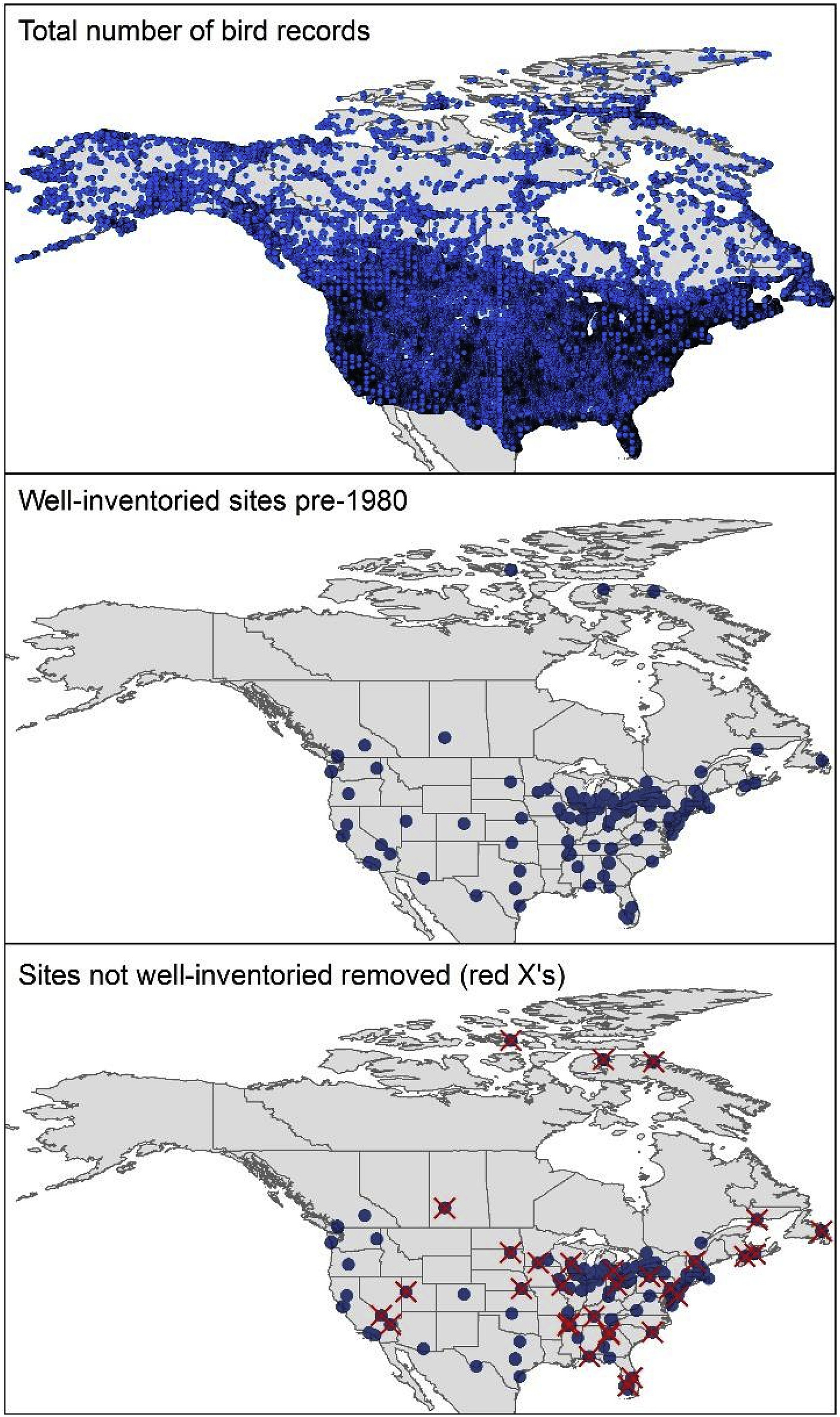
We took advantage of the enormous primary biodiversity data resources available via online data portals, which are integrated and shared via the Global Biodiversity Information Facility (GBIF; Gaiji et al., 2013). We downloaded 4,843,222 GBIF records corresponding to birds from the United States and Canada until 1980, from which 2,735,408 were eBird records (Fig. 2, top panel; see Appendix). We then implemented a series of data cleaning steps designed to assure that the data used in our analyses would be as error-free as possible, since errors and inconsistencies are known to reduce metrics of inventory completeness (Sousa-Baena et al., 2013; Khalighifar et al., 2020).

Figure  2.  Summary of data inputs (blue dots, top panel) along with well-inventoried sites in the past dataset (middle panel; n ​= ​139 blue circles), and well-inventoried sites in the past and present datasets (bottom panel; n ​= ​108 blue circles). Sites with completeness values less than 0.9 are shown as red X's (n ​= ​21).

DownLoad: Full-Size Img PowerPoint

We removed all records with BasisOfRecord ​= ​“fossil specimen,” “machine observation,” or “unknown.” For time, we decided to use “day” as a unit of effort. We isolated data on day, month, and year, and filtered data records to remove any months outside of the integer range of 1–12, and any day numbers outside the appropriate number of days for that month. We removed all records with year ≤1800 (Fig. S1). Finally, we created a unique time marker in the format “YYYY-MM-DD,” which was used to identify individual sampling days uniquely in analyses of incidences.

Regarding sites, we filtered records based on the existence of geographic coordinates and on coordinate uncertainty, retaining only those records including coordinates with an associated uncertainty value of ≤10 ​km. We next assessed whether the coordinates fell within the United States and Canada, discarding marine records and records from elsewhere in the world. Next, we checked that the geographic coordinates fell within the state or province that was (in most cases) given with the record — any records that were markedly misplaced (e.g., not sitting right on the border between two adjacent states) were discarded. Finally, we related the geographic coordinates of the 156,569 localities (many with multiple species records associated) to a 0.05° “fishnet” (QGIS Development Team, 2016) covering all of the United States and Canada, and used the identification number field of this network as an identifier of site in our analyses.

Taxonomy was more complicated to manage. We began by removing records with species names that were unclear or missing, and any taxa that are not known to occur in the United States or Canada or that occur only as rare vagrants. Given that the GBIF data come from different institutions that employ distinct taxonomic arrangements, we compared the set of names in our working dataset against a series of taxonomic authorities to find a best match (i.e., Peters, 1931–1987; Morony et al., 1975; AOU, 1983, 1998; Sibley and Monroe, 1990). The best match was found with intermediate-age authorities: 2344 species for Peters (1931–1987), 2586 for Morony et al. (1975), 2625 for Sibley and Monroe (1990), 2187 and 2275 species for AOU (1983, 1998), respectively. We selected the Sibley and Monroe list, representing what is likely a best balance between being modern enough to include many elements of current taxonomic opinion, but also a list that is not so new as to include massive numbers of splits, which would be hard to get right without, for instance, re-examining many specimens. Species lists were inspected to fix synonyms, misspellings, and other problems.

Records were checked against the distribution of each species (Alderfer and Dunn, 2014) to correct for names that, even though exact, refer to different taxa (e.g., recent split), with some records being removed. Previous simulation studies suggest that, for a suite of estimators, even low frequency errors in large datasets can affect inventory completeness estimation (e.g., Chao 2; Khalighifar et al., 2020). In the end, starting with 4,843,222 records, we were left with 3,720,250 specimen and observational records. Removing records for which identifications were either uncertain or likely wrong, we had 3,523,936 records. Finally, under the Sibley and Monroe taxonomy, and removing duplicate records (i.e., returning unique combinations of species, day, and site), we were left with 3,073,785 records of 673 species.

2.2   Inventories pre-1980: completeness analysis

For computational simplicity, we conducted completeness analyses in Microsoft Access. Specifically, for each of the initial 156,569 sites, we used information on species identification and time (day) to count the: (1) number of unique data records (i.e., combinations of time and species, termed N); (2) number of species known to be present at the site (termed S_obs); (3) number of species recorded on one day only (termed Q₁); and (4) number of species recorded on exactly two days (termed Q₂). With this information, we were able to apply the “Chao 2” equations to estimate S_exp, the number of species expected to be present at the site (Colwell, 1994–2016; Colwell and Coddington, 1994), as $S_{\text{exp}}=S_{\text{obs}}+\left(\frac{N-1}{N}\right)\left(\frac{Q_1\left(Q_1-1\right)}{2\left(Q_2+1\right)}\right)$.

We calculated inventory completeness as C = S_obs/S_exp (sensu Peterson and Slade, 1998), which estimates the proportion of the total avifauna present in a given place that has been detected so far. We used a criterion of C ​≥ ​0.9 for choosing sites for further analysis. In view of occasional sites that have artifactually high values of C, however, to assure inventory quality, we also required that sites have N/S_obs > 10. This pair of requirements reduced our initial list of localities to 139 sites that were demonstrably complete in terms of their inventories (referred to hereafter as “well-inventoried” sites), which summarizes the state of knowledge of avifaunas from the United States and Canada before 1980.

2.3   Inventories post-2010

Because the number of observational records of birds from the United States and Canada post-2000 is enormous (∼3 ​× ​10⁸), obtaining and analyzing the entire dataset was not feasible. As such, we restricted eBird queries to post-2010 (i.e., 2010–2016), which reduced the overall dataset by about 20%. We also created a 50-km buffer around each of the 139 well-inventoried sites in terms of its avifauna prior to 1980, and used the bounding coordinates of these areas as probes into the eBird dataset. Just in the regions close to our well-inventoried sites, we had 25,333,578 records available, such that the dataset was still quite large. We partitioned this overall dataset into 139 files, corresponding to each of the pre-1980 well-inventoried sites; these files varied significantly in size, with as few as 100 records, and ranging up to more than a million records.

To make these data consistent with the pre-1980 analyses, we imposed a series of translations and filters. First, we reduced the original 1133 distinct scientific names to 616 names, based on synonyms and clear identification errors, and translated all names to the Sibley and Monroe authority list. Next, we filtered the data to remove records for which the field “complete checklists” was not equal to 1, and records for which the “effort distance” field was ≥5 ​km. As a final control on data quality, we used the BirdLife/IUCN range polygons (BirdLife International, 2015) for North American birds to remove records of vagrants, and — more importantly — erroneous reports from the dataset. We filtered records of each species based on how close they were to the range polygon for that species, and removed records that were >50 ​km from the range polygon. Although this step removed only a small proportion of records from the dataset, it was nonetheless important in cleaning out errors that elevate Q₁ particularly, therefore reducing estimates of C. At the end of all of these filters, we had 19,334,800 records for analysis.

Owing to the still-very-large nature of this remaining dataset, and the smaller number of sites involved, as compared with the “before” data, we conducted the completeness analyses in EstimateS (Colwell, 1994–2016). Previous experience has indicated to us that calculations of S_exp in Access (above) and in EstimateS are equivalent, so we are comfortable with this difference in methodology. Because EstimateS has a limitation to ∼2500 days of sampling, for 46 sites that had >2500 days of sampling, we took random subsamples of 2500 sampling days with 10 replicates from each site, and used the output to calculate S_exp in EstimateS. We calculated C as described above.

2.4   Summary analyses

Once we had identified the set of sites for which the pre-1980 inventories were complete (n ​= ​139), and the subset for which post-2010 inventories were also complete (n ​= ​108), we compiled a before-and-after table of species ​× ​site. This table had 0 (absent from both inventories), 2 (present in both inventories), 1 (“gains,” absent pre-1980, present post-2010), and −1 (“losses,” present pre-1980, absent post-2010) values, holding a total of 601 species, and formed the basis for all subsequent analyses (Table S1). Final numbers of occurrence records were 3 ​× ​10⁶ and 1.9 ​× ​10⁷, for pre-1980 and post-2010 inventories, respectively. From these occurrence records, we created species accumulation curves for each of the 139 sites to illustrate potential differences between both datasets (Fig. S2). We summarized the before-and-after table via a Jaccard index, in which avifaunal turnover between the two time periods was calculated as (gains ​+ ​losses)/(both ​+ ​gains ​+ ​losses). This index can be interpreted as the proportion of species entering and/or leaving the avifauna over the total species pool ever recorded at that site (i.e., turnover). Species may be present but undetected in a sample (MacKenzie et al., 2002), but we do not envision the probabilities of those nondetections as changing through time, at least not by much, such that, because observer effort in generating the “after” dataset was much greater than that in generating the “before” dataset, many species will have been recorded in the “after” dataset that may well have been present but unrecorded in the “before” dataset. For this reason, we also assessed the proportion of species lost from the inventory, as these losses will be particularly well established in our analyses, compared to species gained.

We assessed the overall spatial autocorrelation in our metrics to determine if spatial signals for turnover or species loss were detectable at a local or continental scale. Specifically, we calculated Moran's I in ArcGIS v10.5.1 (ESRI, 2016), an index of spatial autocorrelation, and compared the observed value to a null distribution derived from randomizing values many times (number not specified by the routines in ArcMap 10.2) across the full set of sites. Finally, we inspected the results taxon by taxon for species-level effects implementing exact binomial tests in R for the number of gains (successes) and losses (failures). We used a null probability of success of 0.5, which assumes that is equally likely to gain or loss a species in any site (Table S1). We looked at both extremes of the probability distribution (i.e., more losses than gains, and more gains than losses), however, due to the reasons of massive sampling bias that were discussed above, we did additional exact binomial tests for the species that showed more losses than gains. In these binomial tests, we increased the probability of success (i.e., gain), given that gains are more likely than losses in our comparisons (Table S2). All species names presented herein are based on Chesser et al. (2020) to maximize relevance to current ornithological work.

As an additional exploration of our approach, we contrasted historical knowledge of avifaunas (pre-1980; compiled by Peterson et al., 2016) against modern eBird data (2010–2020; Appendix) for Chichén-Itzá, Mexico. The pre-1980 completeness analyses were developed using the same methodology as that employed in our analyses for the United States and Canada described above, and indeed were executed by the same individual (Peterson). We downloaded the eBird data for this one locality using the R package auk (Strimas-Mackey et al., 2018), and processed, cleaned, and filtered the data through the same process as described above (Appendix 2), with completeness analysis being carried out via the same means as well. Doing a before-and-after comparison for this well-inventoried site, we offer new insights on avifaunal turnover for a locality lacking time series data, and highlight the importance of our approach in biodiversity-rich regions.

2.5   Potential drivers of avifaunal change

To determine potential causes of the patterns of detected avifaunal loss, we explored the relationship between our initial results and the degree of observed land cover change and climate change. To analyze land cover change, we used the Global Land Surface Satellite climate data records (GLASS-GLC), which are categorized in 7 classes (e.g., forest, grassland, tundra) at 5 ​km spatial resolution from 1982 to 2015 (Liu et al., 2020). Climate data were obtained from the National Center for Environmental Information at ∼6 ​km spatial resolution (Livneh et al., 2015). These climatic data consisted of interpolated raster layers of temperature and precipitation created using meteorological data from weather stations across North America for the period 1950–2013. We note that the temporal intervals of focus (i.e., pre-1980 versus post-2010) do not coincide precisely with the temporal intervals in land cover and climate layers, but these data products had the closest temporal match that we could find at this level of spatial detail.

We assessed changes in forest cover and climate by buffering all well-sampled sites by a distance of 50 ​km. To depict forest cover change, we considered two variables: (1) proportional area (in pixels) per buffer that presented forest loss (FL) and (2) proportional area of each buffer that presented forest gain (FG), between the earliest (1982) and most recent (2015) layers of the GLASS-GLC dataset using the CROSSTAB module in Terr Set 2019. To represent climate change, first, we divided the data into two periods 1950–1980 (before) and 2010–2013 (after), and analyzed the change between them. From these analyses we created two variables: (1) proportional area of each buffered site where mean temperature increased (ATI); and (2) proportional area of each buffered site where precipitation increased (API). Proportional areas of each buffered site where temperature and annual precipitation decreased, ATD and APD, were highly correlated with ATI and API (ATD-ATI r² ​> ​0.9, APD-API r² ​> ​0.9), and were not included in our models to avoid multicollinearity issues. Raster procedures were performed using ArcGIS.

To account for spatial autocorrelation, we ran a Principal Coordinate Analysis (PCoA) of the sites geographic distance matrix, and included the eigenvectors as part of our predictor variables. With this approach one can decrease the influence of spatial autocorrelation in macroecological analyses, and account for broad- and fine-scale spatial variation through eigenvectors derived from large and small eigenvalues, respectively (Diniz-Filho and Bini, 2005). Before performing the PCoA, the matrix was truncated (i.e., distances >1000 ​km were multiplied by 4) to give more weight to short-distance effects as recommended by Diniz-Filho and Bini (2005). We selected the first three eigenvectors using a broken-stick method (Diniz-Filho et al., 1998) since they represented most of the geographic and regional relationships of the sites analyzed (Figs. S3 and S4).

To estimate the influences of these factors on avifaunal change, we performed multiple linear regression analyses of species loss as a response (log-transformed) to four predictors (FL, FG, ATI, API), and three eigenvectors (E1–E3). We ran a total of 30 distinct candidate models, using as predictors all potential combinations of the four environmental variables, with and without variable interactions, and including the three eigenvectors in all models. We selected the best models using the Akaike Information Criterion difference (ΔAIC), retaining models with ΔAIC <2 and testing statistical significance of driver effects using F tests.

3.   Results

We identified a total of 139 well-inventoried sites in the pre-1980 data (i.e., inventory completeness >0.9), which were concentrated in the eastern and midwestern United States and southernmost Canada, but included three high-Arctic Canada sites and scattered sites in the western United States (Fig. 2). Of these 139 sites, 108 were also well-inventoried among post-2010 data, such that the great majority of the historical sites were also well-documented in the present dataset (Fig. 2; Table S3). Accumulation curves for such sites usually stabilized between 1960 and 1980, with most of them showing slight increments in the post-2010 dataset, relatively to the observed patterns in the pre-1980 data (Fig. S2), hence, we consider our completeness criterion appropriate for site selection. Because the three high-Arctic sites were not among the “after” well-inventoried sites, the footprint of our analyses was reduced to the Lower 48 United States and adjacent parts of southern Canada.

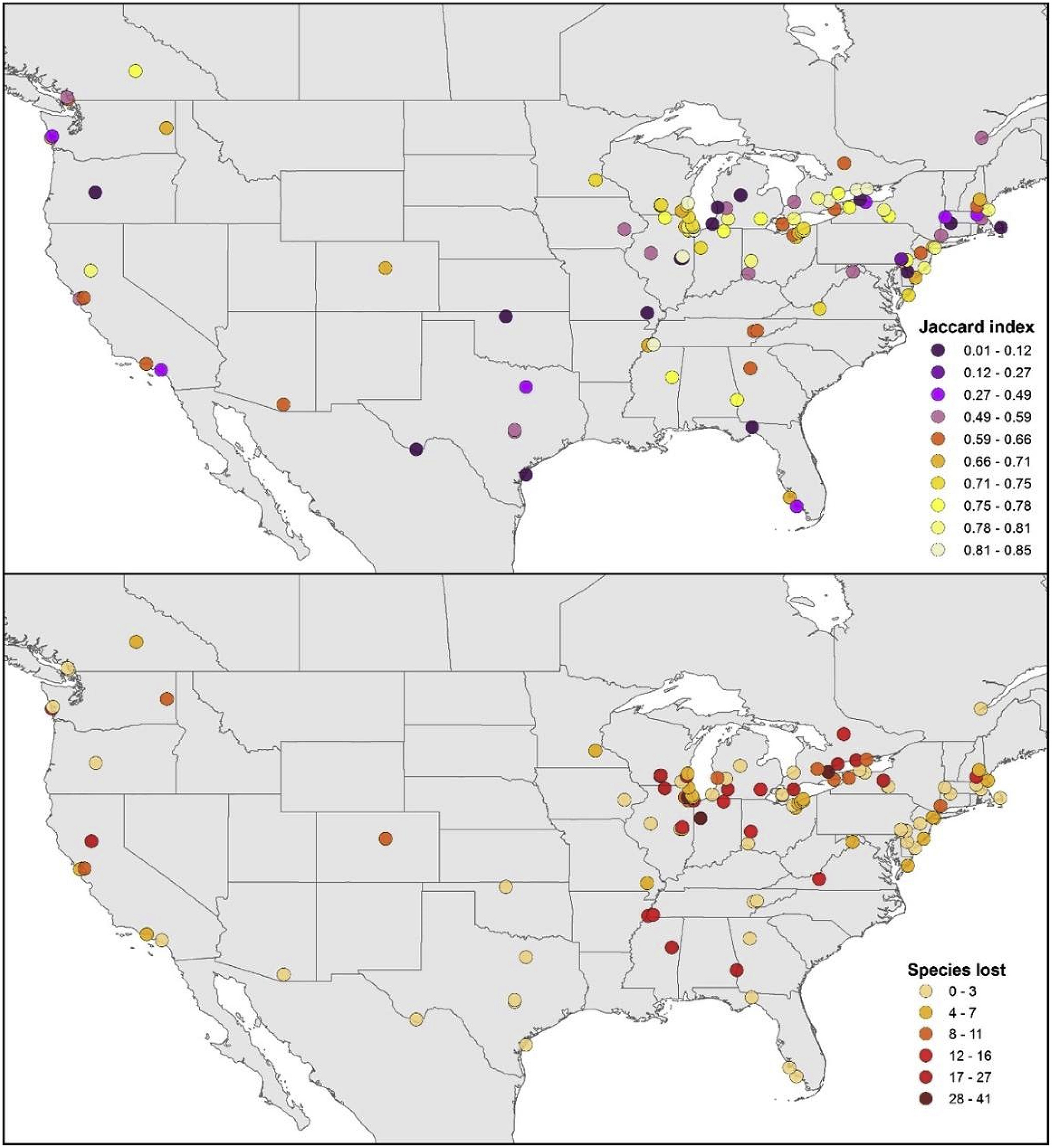
Our turnover measure showed broad differences among sites (i.e., Jaccard index; Fig. 3), and through an eigenvector approach we summarized the spatial relationships of sites at continental (eigenvectors 1 and 2; E1–E2) and regional (eigenvector 3; E3) scales (see Section 2.5. Potential drivers of avifaunal change; Fig. S3). Sites in the northeastern region of our study area showed higher values for turnover and species loss metrics. Overall, turnover ranged 0.01–0.85, with highest values at sites in the midwestern and northeastern United States, and lowest values scattered across Oregon, Oklahoma, Missouri, Texas, Florida, Illinois, Michigan, New York, Massachusetts, and Delaware. Species losses in local inventories ranged 0.0–16.0%, with highest losses at sites around the Great Lakes, the southern United States, and northern California, and lowest losses again scattered throughout the northwestern, southern, and parts of eastern United States. Spatial autocorrelation analyses of these metrics were positive (i.e., clustered spatial patterns are present; Moran's I), with significant results for overall species turnover (Z ​= ​2.5, P ​< ​0.05) but without species loss being different from null expectations (Z ​= ​0.74, P ​= ​0.457).

Figure  3.  Summary of overall patterns of species turnover (top) and species losses (bottom) across 108 sites for which inventories were complete for both pre-1980 and post-2010.

DownLoad: Full-Size Img PowerPoint

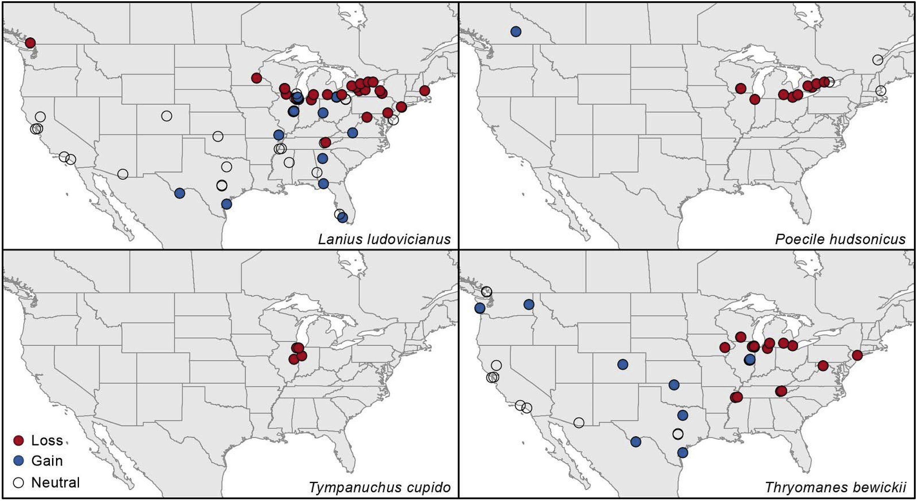
Our species-level assessments revealed a number of interesting trends. For instance, we noted two species for which loss/gain binomial tests were statistically significant: Poecile hudsonicus (P ​= ​0.012) and Lanius ludovicianus (P ​= ​0.038; Fig. 4). A further set of species showed a tendency for losses to outnumber gains, which we explored owing to a far-greater probability of detection in the “after” time period in our datasets (see Section 2.4. Summary analyses), even though binomial tests with a probability of success (i.e., gain) of 0.5 were nonsignificant (Table S1). These species were Pinicola enucleator, Coccothraustes vespertinus, Picoides arcticus, P. dorsalis, and Thryomanes bewickii (Fig. 4), which are mostly boreal. Increasing the probability of gain for additional binomial tests in this species subset showed statistically significant results for all species (Table S2). An additional species showing significant losses in present inventories at the northern limit of its distribution was Rallus elegans (Table S2). Moreover, we highlight that the Greater Prairie-Chicken, Tympanuchus cupido, showed 4 losses in Illinois and Indiana against no gains in present records (Fig. 4). At the other end of the spectrum (i.e., gains outweighing losses), we noted the following taxa: Grus americana (17 gains to 1 loss), Corvus corax (40 gains to 2 losses), Bubulcus ibis (51 gains to 3 losses), Setophaga kirtlandii (10 gains to 3 losses), and Quiscalus mexicanus (11 gains to 0 losses), with the first three species showing significant results in binomial tests (Table S1).

Figure  4.  Patterns of loss and gain at sites with complete inventories in both pre-1980 and post-2010 for four example species. These species showed statistically significant binomial tests (see ), with the exception of T. cupido given sample size (no sites with gains).

DownLoad: Full-Size Img PowerPoint

Relating species loss rates to possible environmental drivers (i.e., temperature, precipitation, forest cover), three best linear models were selected out of 30 candidate models (Table 1). All models included the proportional area of precipitation increase (API) and the third spatial eigenvector as significant predictors, although the latter variable had a considerable small coefficient (−9 ​× ​10⁻⁷; Table 1). These models suggest that avifaunal losses at sites studied rose in areas with increasing precipitation. Two of the three models exhibited interaction predictors of precipitation and temperature (API∗ATI) and precipitation and forest gain (API∗FG), that were almost significant (Table 1; see Section 2.5. Potential drivers of avifaunal change).

Table  1.  Coefficients for the intercept (B) and the predictors of best general linear models for log species loss, selected based on the Akaike Information Criterion difference (ΔAIC) values.

ΔAIC	df	B	E1	E2	E3	API	ATI	FG	API∗ATI	API∗FG
0	8	−13	7 × 10−8	6 × 10−8	−9 × 10−7	12.8	7.0	−	−11.4a	−
0.76	6	−7	8 × 10−8	8 × 10−8	−9 × 10−7	2.3	−	−	−	−
1.30	8	−8	6 × 10−8	9 × 10−8	−9 × 10−7	3.5	−	24.3	−	−28.2b
Significant predictors (F-tests) are shown in bold. Column titles are abbreviated as df: degrees of freedom; E: eigenvectors (E1–E3); API: proportional area of buffered site with increased precipitation; ATI: proportional area of buffered site with increased mean temperature; FG: forest gain.
a P-value = 0.053.
b P-value = 0.073.

 | Show Table

DownLoad: CSV

Our before-and-after comparison of 265 species in Chichén-Itzá (Mexico), a site within a biodiversity hotspot (i.e., Mesoamerica; Myers et al., 2000), was included to illustrate how these before-and-after comparisons can inform about regions that may be less intensively sampled. These analyses revealed likely species losses (e.g., Patagioenas speciosa has no recent records, but was present among the older records) and gains (e.g., Polioptila bilineata is not represented in the pre-1980 sample, but has been recorded by multiple observers recently), vagrant species (e.g., Coereba flaveola, which is represented by a few records in the recent dataset, but is likely not resident, given their sparsity), as well as recent invaders (e.g., Streptopelia decaocto, a Eurasian species that arrived in the Americas after 1980). Finally, 24 aquatic and wetland species have been reported recently that were not registered in Chichén-Itzá before 1980 (Table S4).

4.   Discussion

This project confirms the potential utility of unplanned, post hoc comparisons among very different sources of primary biodiversity data in characterizing biodiversity change. Our analyses recovered range wide patterns of population decline in a number of species for which their range and population reductions had been noted in the literature previously. Our analyses also documented northward range retractions in several boreal species, a result that matches the expectations from general patterns of species’ responses to climate warming processes (Parmesan et al., 1999; Parmesan and Yohe, 2003; Peterson, 2003). As such, in spite of a number of caveats and complications (see discussion of these issues below), we see considerable promise for those cross-data-stream, longitudinal comparisons of avifaunal composition.

Our results illustrate the broadening potential for synthetic analyses to be constructed on top of large-scale biodiversity information resources. Although other studies have approached some of the same questions (Peterson et al., 2015; Jarzyna and Jetz, 2017; Spooner et al., 2018), here we have integrated massive amounts of data (i.e., 3 ​× ​10⁶ pre-1980 and 2 ​× ​10⁷ post-2010 records) to characterize avifaunal turnover in decadal times, and explored potential associations of biotic change with local and broad-scale factors for more than half of the species of continental U.S. and Canada (601 species). The integration of detailed biodiversity data from specimen collections and massive observational data resources over a span of decades demanded different data manipulations and analytical steps. As such, this project is a novel demonstration of emergent properties that become visible and obtainable only when critical masses of data are created, made digital, and made openly accessible. Furthermore, the present study sets guidelines for research in biodiversity hotspots where time series data are limited or nonexistent, but complete inventories for different time periods are available.

4.1   Drawbacks and caveats

Although we took great care to assure good data quality for both of the time periods in our inventory assessments, we must note particularities of each period that can make for problems in interpretation of our results. Part of the “before” sample was derived from specimen collections, which involve laborious steps of obtaining the individual bird, preparing and conserving the specimen, capturing the relevant data, and making the data available. Certainly, some taxa are far more easily collected and prepared than others: a warbler or a blackbird is far more likely to appear in the “before” lists than a vulture or a swan, among other biases inherent in museum specimen data (Reddy and Dávalos, 2003). Indeed, as larger-bodied birds can require even days of effort for preparation, not only may they not appear in the older inventories (depressing the number of observed species, S_obs), but they also are far more likely to be represented by single records, rather than multiple records, which depresses the completeness measure (C) in our calculations. Collectors also have biases in on which species they focus their attention, and their collection efforts, concentrating on locally abundant or range-restricted species; these biases may affect the representativeness of their collections.

The observational data that dominated our “after” sample have some different characteristics, as they derive from community-science efforts that are not conducted systematically. Clearly, observers are often quite sophisticated, and can gather massive quantities of data and report them in short order. In this way, truly large-scale data resources can and have been assembled for much of our study area. Although observational data certainly benefit from large sample sizes, they can also hold more errors and noise, which in many cases cannot be revisited or rechecked (Bonney et al., 2009; Sullivan et al., 2009). Those errors can act to create single records, which elevate the number of expected species (S_exp) and reduce C. In the end, however, the five-fold greater volume of data, as well as the collecting biases mentioned above, act to make the species lists in the post-2010 dataset more complete, such that we have emphasized losses (i.e., non-detection in spite of far-greater sampling effort) more than gains of species at sites in our evaluation and assessment of these data.

4.2   Species-level assessments

Perhaps the most interesting insights of this study emerged from our species-by-species assessment of changes that occurred after the considered 30-year time interval. Five boreal species of Canada and Alaska showing significantly more losses than gains, have ranges extending only marginally into the region that was covered by our network of well-inventoried sites. This set of five species represents 19% of ∼28 species of boreal distribution. Therefore, our work appears to be reflecting a northward retraction of a suite of species with southern range limits at the northern border of the Lower 48 United States.

Recently, it has been shown that the largest decrease in bird abundance has been suffered by species that overwinter in temperate North America (Rosenberg et al., 2019). For Poecile hudsonicus in particular, Breeding Bird Survey data shows negative trends along the United States-Canada border (Sauer et al., 2017a), where our data suggest range loss for that species (e.g., Michigan, Ontario, Wisconsin). However, the detection of patterns can depend on the species and the design of surveys and monitoring schemes (e.g., riparian species counts might be underestimated by Breeding Bird Survey routes; Robbins et al., 2010), and for instance, P. hudsonicus has been considered irruptive in the state of New York outside the Adirondack Mountains (Yunick, 1984). We acknowledge that our design might be limited to discern such patterns of irruption, which constitute irregular but repeated movements outside the range of a species (Koenig, 2001). Such patterns have been shown by Christmas Bird Count data for some of the studied boreal species (i.e., P. hudsonicus, C. vespertinus, P. enucleator; Koenig, 2001), and we cannot discard that our results reflect a decrease in irruptions. However, since these events occurred with certain regularity (i.e., these are not accidental species sensu Grinnell, 1922), we explored the implications of our before-and-after comparisons given the massive amount of observations in the post-2010 dataset.

The remaining considered species for which losses were dominant were all species for which rangewide population declines had previously been noted and assessed: Tympanuchus cupido has retracted from major sectors of its historical range (Mussmann et al., 2017), which is part of its massive range and population collapse. Lanius ludovicianus has shown precipitous population declines over much of its range, possibly related to both habitat loss (Cade and Woods, 1997) and climatic factors (Illán et al., 2014). Northern populations of Rallus elegans have exhibited long-term declines caused by land cover change and wetland degradation (Cooper, 2008), although we acknowledge that this species is secretive and seems to be more scattered in the Midwest and around the Great Lakes. Finally, Thryomanes bewickii also has shown massive population declines, at least across the eastern portion of its distribution (Smith, 1980; Kennedy and White, 1996).

We have singled out a few species for which we believe that the “gains” may prove to be biologically meaningful. That is, we found gains outnumbering losses rather impressively in Setophaga kirtlandii and Grus americana, which in both cases correspond to at least modest recoveries in species that were formerly on the brink of global extinction (Servanty et al., 2014; Brown et al., 2017). Although our detections are not necessarily of breeding populations, we suspect that observational documentation of their presence at sites since 2010 reflects overall greater numbers of individuals, at least in part. However, we cannot discard that the lower collecting pressure on these species, which were quite rare pre-1980, might also generate the observed pattern. Large numbers of gains in Bubulcus ibis and Quiscalus mexicanus reflect the massive range expansions that both species have manifested in their distributions (Wehtje, 2003; del Lama and Moralez-Silva, 2014). Finally, the concentration of range gains in Corvus corax in the eastern portion of its range is concordant with recent population recovery there (McGowan and Corwin, 2008; Sauer et al., 2017b). Certainly, in some cases, other patterns could not be discerned for lack of sufficient points in certain regions of North America (e.g., U.S. western half, central and northern Canada).

This set of species illustrates how before-and-after comparisons can detect population and range trends that have been also noted from different types of data (e.g., long-term monitoring schemes, population abundance data), providing a degree of independent confirmation. Since knowledge of the distribution and trends of biodiversity is spatially biased (Fig. 1; Yesson et al., 2007; Collen et al., 2008; Dornelas et al., 2018), we present our approach as a way to explore changes in assemblage composition in important areas (e.g., biodiversity hotspots), where occurrence data, either from scientific collections or observational sampling, are available to develop before-and-after comparisons over long time scales.

It is tempting to dismiss these approaches as something that can be done only in regions that have been sampled intensively. For that reason, we explored the example of Chichén-Itzá, which had been documented in previous analyses as well documented in terms of its avifauna prior to 1980 (Peterson et al., 2016). Our before-and-after analysis revealed a mostly stable avifaunal composition, but also detected several changes that are intriguing, such as the likely loss of the tall-forest-associated pigeon, Patagioenas speciosa from the local avifauna. Although the approaches that we have explored characterize only single points, or local landscapes, and may not offer continuous coverage across entire regions (Peterson et al., 2015), they also avoid the complicating effects of broad data aggregation over space, and the consequent confusion of alpha- and beta-diversity. As such, we offer these methods as means of obtaining some information for regions where none would be available otherwise.

4.3   Potential drivers of avifaunal change

Our assessment of whether a broad-scale, autocorrelated signal exists in overall species turnover or in proportional loss of species at sites is interesting, but possibly also frustrating. In particular, that turnover is indeed positively autocorrelated, but species losses are not, suggests that this result might be an artifact of greater detection and larger numbers of species gains at many sites. Additionally, the non-significance of the species loss spatial autocorrelation may also be a consequence of the low overall variation in species loss, which is not marked, such that the metrics based on this dataset may not be sensitive. However, if both signals of positive autocorrelation were real (Fig. 3), these patterns would reflect changes in assemblage composition at a regional scale, this is, the Great Lakes region of both countries and northeastern United States (see below).

Our analyses of potential drivers of avifaunal loss in the sites studied revealed that losses were positively related to areas where precipitation increases in all models. Interactions among drivers had relatively strong effects, but were nonsignificant. Although precipitation changes can be region-specific, precipitation has been considered a factor of North American birds range boundaries (Root, 1988b), and has increased globally at least since the 1980s (Wentz et al., 2007; Lambert et al., 2008). Moreover, precipitation change, coupled with raising temperatures, has been proposed as a main driver of distribution changes in birds from western North America (Tingley et al., 2012; Illán et al., 2014). The proportional area of precipitation increase (API) does not directly reflect mean change in precipitation in each site, but it is an indicator of how precipitation has changed in the time interval considered. Interactions among temperature, precipitation, and land cover change have also been suggested to generate biotic change (Higgins, 2007). However, our evidence is not strong enough to establish whether interactions among predictors also constitute significant drivers of avifaunal losses in our study area.

Global warmer temperatures increase evaporation and radiative cooling of the atmosphere, which increases latent heating and precipitation (Lambert et al., 2008; Previdi and Liepert, 2008; Collins et al., 2013). Likewise, northern mid-latitude afforestation (i.e., forest gain) has the potential to change the regional energy budget, increasing surface temperature due to a lower albedo, but also to shift global precipitation belts northwardly (Swann et al., 2012). Our results are particularly relevant for mid-latitude sites in the Great Lakes region of both countries and in northeastern United States, due to the imbalance of available data. The inclusion of eigenvectors as predictors in our models aimed to remove autocorrelation biases from significance tests of the regression coefficients (Diniz-Filho and Bini, 2005). Hence, we think that the increase in precipitation is associated with some of the observed biotic changes in this region. In fact, recent research using weather radar information shows a consistent trend in bird biomass reduction across eastern United States (Rosenberg et al., 2019), where precipitation has indeed increased (Easterling et al., 2017).

5.   Conclusions

This project is, in many senses, presented as an exploration and a proof of concept, and resulted in an intriguing set of insights into distributional change in the North American avifauna. Although birds in the United States and Canada are perhaps a special case, in which both collecting and observational effort have been particularly intensive, they are far from the only case in which before-and-after comparisons can be developed, and rapid accumulation of primary biodiversity data resources worldwide is making such analyses possible in many more areas of the world. We show that, even in these countries, there are still places for which knowledge on species distribution and assemblage composition can be improved (e.g., midwestern and western United States; see Table S3 for potential sites needing modern sampling efforts). In that sense, historical collections resources can and should be inspected for well-inventoried sites. These sites may be field stations, historical points of access, residences of particular researchers or collectors, national parks, or other places that for whatever reason were sampled intensively in the past (Moritz et al., 2008; Tingley and Beissinger, 2009, 2013; Rowe et al., 2014; Cavarzere et al., 2017). Resampling a single site for which historical information exists is rewarding in that the before-and-after comparisons on a local level can be interesting and useful, as we have shown for Chichén-Itzá, and such efforts can be carried out on large scales with the “power of numbers” that becomes possible with the involvement of citizen-scientists. However, resampling a suite of such sites offers a multi-scale view of biotic change, such that the gap in temporal scales of biodiversity studies can feasibly be filled.

Author contributions

ATP conceived the study; FMS, BF, MEC, CNP, LJ, UP, AK, WT, TDS, SF, and LOO collected data and conducted research; FMS, BF, DJG, MEC, CNP, LJ, EK, AK, KI, and LOO developed methods and analyzed data; FMS, BF, MEC, LJ, and ATP wrote the paper. All authors read and approved the final manuscript.

Declaration of competing interest

None.

Acknowledgements

We thank the remaining members of the KU Ecological Niche Modeling Group for their support and assistance in various phases of this project. In particular, we thank Jorge Soberón and Mark Robbins for wisdom and guidance in aspects of the analyses reported herein. FMS wants to express his gratitude to Pietro de Mello and the WOG group for their support throughout this project.

Appendix A.   Supplementary data

Supplementary data to this article can be found online at https://doi.org/10.1016/j.avrs.2022.100005.