Figure
1.
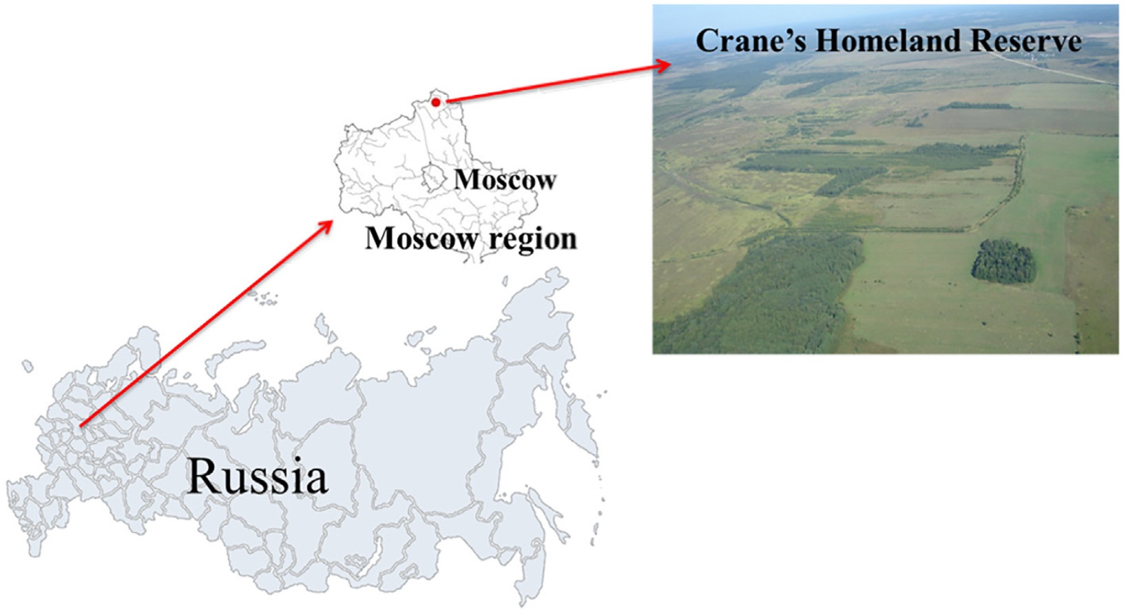
Map of study site.
| Citation: |
Tatyana Kovinka, Alexander Sharikov, Tatyana Massalskaya, Sergey Volkov. 2023: Structure and heterogeneity of habitat determine diet of predators despite prey abundance: Similar response in Long-eared, Short-eared Owls and Common Kestrels. Avian Research, 14(1): 100072. DOI: 10.1016/j.avrs.2022.100072

|
According to one of the theses of optimal foraging theory, main prey species abundance in the hunting area is the main factor determining the diet and habitat choices of birds of prey. However other factors can also be important. The habitat structure influences the predators' diets as well. In this study we examined the influence of habitat structure on diet compositions of three species of birds: Long-eared Owl (Asio otus), Short-eared Owl (A. flammeus) and Common Kestrel (Falco tinnunculus). The study was carried out from 2007 to 2019 in a 48 km2 area of the Crane's Homeland Reserve, Moscow Region, Russia. The habitat structures of model species' hunting territories (ratio of different types of landscape elements) were classified in module "Semi-Automatic Classification Plugin" based on the QGIS. A boosted regression tree analysis identified that the share of the main prey species in the diet is primarily determined by the landscape structure of hunting territories. The largest share of Common Vole (Microtus arvalis) in birds' diet was determined by the shrubs area (15% of hunting area), the meadow area (75%), the habitat heterogeneity (70%) and the arable land area (5%). The same predictors determined the largest share of Root Vole (Microtus oeconomus): the shrubs area 25%, the meadow area 70%, and the arable land area 3%. The annual mean abundance of prey species did not determine their importance in the diet of birds of prey. Thus, the main prey abundance in the hunting area is not a determining factor for the formation of diet composition of birds of prey.
The diet compositions of birds of prey are relatively plastic (Hobart et al., 2019). Many different factors in the habitat structure can lead to changes in the trophic interactions between predator and prey (Hobart et al., 2019). According to the optimal foraging theory, predators choose the most favorable habitats for hunting to minimize energy consumption (Pyke, 1984). On the one hand, they choose habitats where the abundance of the main prey species is the highest. This factor is important and can determine diet composition of birds of prey (Davorin, 2009). For example, the Long-eared Owl's (Asio otus) diet composition varies from year to year depending on the main prey species abundance. In the years of low Common Vole (Microtus arvalis) abundance, its share in the owls' diet is minimal, and the share of alternative prey increases (Korpimäki, 1985, 1992; Korpimäki and Norrdahl, 1991). However, in some cases the predators' diet composition is not determined by the prey abundance. Other environmental factors are often important as well. Particularly, deep snow and low temperatures reduce the availability of the main prey species and cause predators to switch to alternative preys (Żmihorski and Rejt, 2007; Romanowski and Zmihorski, 2008; Sharikov and Makarova, 2014; Selçuk et al., 2017).
On the other hand, according to the foraging opportunity hypothesis, by which high habitat heterogeneity is commonly associated with higher fitness and expectably with higher diet diversity. It is well known that the diversity of the wildlife increases with the habitat heterogeneity and its resources increasing (Tews et al., 2004). As habitat heterogeneity increases, the proportion of edges and the diversity of small mammal fauna also increases which may be advantageous for birds of prey (Butet et al., 2006). Habitat heterogeneity of hunting territories affects the composition of small mammals' communities and the availability of certain prey species (Kodzhabashev et al., 2020). In each habitat with a certain type of vegetation, predators use different optimal hunting methods (Wuczyński, 2005). For example, Common Buzzards (Buteo buteo) hunt from the ground in territories lacking high and dense vegetation. Moreover, these habitats are often characterized by the best food supply, where high raptor concentrations are also observed. Thus, the hunting territory landscape structure can be an important factor for formation of birds of prey diet composition.
Recent studies have shown a positive relationship between the diversity of owls' diets and the landscape complexity of hunting areas. The presence of open patches with low vegetation is positively associated with the proportion of Microtus voles in owls' diets (Romanowski and Zmihorski, 2008; Milchev, 2015; Szép et al., 2017, 2018). Szép et al. (2017) established a relationship between the abundance of the main prey species in the Barn Owl (Tyto alba) diet and the landscape structure of owls' hunting territories. The abundance of Wood Mouse (Apodemus uralensis) was positively correlated with high landscape heterogeneity. The abundance of the Lesser White-toothed Shrew (Crocidura suaveolens), Water Shrews (Neomys anomalus), Field Mouse (Apodemus agrarius) and Harvest Mouse (Micromys minutus) was higher in more homogeneous territories. The landscape heterogeneity can influence prey diversity in diets. It is interesting that prey diversity in Common Kestrel (Falco tinnunculus) diet increased not by choosing a more diverse landscape, but rather by actively searching for prey in homogeneous territories (Navarro-Lopez and Fargallo, 2015).
Long-eared Owl, Short-eared Owl (Asio flammeus) and Common Kestrel are widespread, co-living and nesting species of birds of prey in open and partially overgrown areas in central and northern Europe, as well as central Russia (Mikkola, 1983; Korpimäki, 1985; Sharikov et al., 2019). These species have a high degree of trophic niche overlap, since in most regions their diet is based on rodents, mainly of the genus Microtus.
We suggest that ratio of different types of habitat elements such as open areas (meadows, arable lands etc.) and areas of forests and shrubs are important predictors determining the raptors' diet. The ratio of these landscape elements can influence prey availability. In open spaces with low bushes hunting will be more successful even if there is low prey abundance compared to with territories with high prey abundance but with dense understory. Thus, the study was aimed at assessing the relative importance of habitat structure versus prey abundance.
The study was carried out from 2007 to 2019 in a 48-km2 area of the Crane's Homeland Reserve (56°45′ N, 37°45′ E), Moscow Region, Russia (Fig. 1). Habitats of the study site were mostly agricultural land (76%), along with some forests and shrubs. Woodlands occupy about 5% of the territory; there are numerous groves and forest belts, represented by uneven-aged tree and shrub associations (16%). In addition, there are a dense system of drainage ditches, small marshes and artificial reservoirs near villages. The habitat structure of study site was significantly determined by nature management. Decrease in agricultural intensity, the processes of forest formation and waterlogging of some patches of study area became significant factors that led to the growth of the unique heterogeneity of the landscape (Grinchenko et al., 2020).
For the diet study of the breeding birds, we collected pellets near active nests and regular roosting places 2–3 times per month from April to June. The determination of pellets belonging was accurate since birds were observed at all nests and roosting places. Nest lining with prey remains was also collected in the end of the field season (August–October). A total of 1474 pellets of Long-eared Owls, 109 pellets of Short-eared Owls and 1785 pellets of Common Kestrels were collected. We processed the pellets and lining in laboratory conditions in accordance with the standard method (Marti, 1976). Identification of prey remains was by upper or lower jaws and pelvic bones (Gromov and Yerbaeva, 1995). Data of the twin-species Common Vole and Southern Vole (Microtus levis) were pooled due to the difficulty of identification by bones; the species pair is hereafter called Common Vole. Bird species were identified by beak and feather remains by referencing the ornithological collection of Department of Zoology and Ecology of the Moscow State Pedagogical University. Insects were identified by remaining chitinous parts. Prey diversity in the diet was estimated using Shannon–Wiener Index (H'; Shannon and Weaver, 1949).
Eight snap-trap lines of 25 traps were set for 3 days in spring (April) and summer (June) (Naumov, 1963; Korpimäki, 1981). In each habitat the traps were situated in a line of 25 traps with an interval of 5 m. Black bread dipped in vegetable oil was used as bait. The snap-trapping lines were situated in different habitats within the hunting territories of birds and were operated for a total of 28,654 trap-nights in 2007–2019. Prey abundance was calculated according to the following formula:
|
X=N×100/M |
where N is the number of caught rodents and M is the number of traps/nights.
We used this method because it allows to accurately determine the species of Microtus voles (determined by the chewing surface of the teeth). Unfortunately, other non-lethal or passive methods do not accurately identify Microtus voles down to species.
A total of 91 nests (23 Long-eared Owl, 10 Short-eared Owl and 57 Common Kestrel) were monitored between 2007 and 2019. We conditionally considered the territory with radius of 500 m around the nest as the hunting territory of the nesting pair. Spatial data for describing habitat in the hunting area were obtained from the US Geological Survey website "USGS" (USGS: U.S. Geological Survey, 2019). We used multichannel images from Landsat satellites 4–5, 7 and 8. For each year we selected one image from the spring (mainly April). If the image for April was poor in quality, we selected the image for May, then for June, and only then for March. For years when the image quality was poor for all of these months, we used an image from the next year. It was considered that there were no significant changes in vegetation during the year. All spatial data were processed in the program "QGIS 3.14" in module "Semi-Automatic Classification Plugin" (Quantum GIS, 2020).
Each habitat type was defined as a separate land cover class. For each type of land cover classes, we created a training shapefile which stores the ROIs (i.e., Regions of Interest) — most typical vegetation area using the vegetation index NDVI. In total, five land cover classes were allocated on the model territory: first class – forest (i.e., continuous forests); second class – shrubs (i.e., fields overgrown with shrubs, forest belts and willows); third – meadow (i.e., herbaceous vegetation); fourth – farmland (i.e., arable land and roads); fifth – rare types of habitats, space image errors, clouds and their shadows. The sixth class was villages. The areas occupied by villages were classified separately, based on their boundaries, determined by the images from Landsat satellite.
We classified Landsat images using a semi-automatic approach (i.e., the entire image is classified automatically based on several samples of pixels "ROIs" that are used as reference classes; Congedo, 2014). Before the classification process, we converted the DN values (Landsat Bands) to reflectance by DOS1 method. DOS1 method provides a simple atmospheric correction for the comparison and mosaic of different satellite images, and improves the classification results (Congedo, 2014). After that we used the "Pansharpening" function to improve image quality for Landsat 7 and 8. This function is available only for Landsat 7 and 8 (Korpimäki, 1981). In order to create the color composite in QGIS we created visual raster. The RGB = 432 (green, red and near-infrared bands) was selected as the color composite of the image (Congedo, 2014). After that we defined the band set that we classified landscape of model territory.
"Land Cover Signature Classification" algorithm was used to classify vegetation. "Spectral Angle Mapping" algorithm was used for unclassified data with a threshold of 0.0. The output was one raster layer containing all five land cover classes (Congedo, 2014).
The classification accuracy was assessed by the "Accuracy" function and varied from 83% to 100%. The classification is considered accurate at a value of 80% or more (Congedo, 2014). The resulting raster classification was generalized to remove very small class areas. The "Classification sieve" algorithm was used with combining of pixels by four and a threshold value of 12 for this. Then the generalized classification raster was converted to vector graphics (Congedo, 2014). Each vector file was transformed by the QGIS Geometry Correction tool to calculate habitat area.
For each hunting territory the total area of five land cover classes was determined and the coefficient of habitat heterogeneity calculated (Vinogradov, 1998).
|
K=mm−1[1−n∑i=1(SiS)2] |
where S is the total land area, Si is the area of contours of i-class vegetation, and m is the number of vegetation classes.
The presence or absence of water and roads was also determined in the hunting area. Moreover, roads were classified in two types: asphalt and unpaved.
We used a machine learning technique for estimation of different predictors' influence on the model species diet composition. The machine learning technique is in contrast to traditional model fitting where the parameters are often estimated based on the assumption of linear and additive relationships. This technique assumes that the relationships between predictor and response variables are complex and determines the relative importance of different predictors by including nonlinear and interactive relationships as well as validating the models (Elith et al., 2008).
To create the models, we used boosted regression trees (BRT) with Gaussian distribution implemented using the gbm (Version 2.1.3) package in R (Elith et al., 2008; R Core Team, 2012). Boosted trees are a statistical learning method that allows both of objectives for regression and classification analyses. They can deal with many types of response variables. Interactions between predictors can also be quantified and visualized (De'Ath, 2007). In the BRT analysis, we chose Gaussian as the error structure for the loss function because of the attribution of our response variable. The fitting of a BRT model is also controlled by the following factors: 1) the learning rate determines the contribution of each tree to the growing model; 2) tree complexity controls the level of interactions in BRT; 3) bagging fraction sets the proportion of observations used in selecting variables; 4) cross-validation specifies the number of times to randomly divide the data for model fitting and validation (De'Ath, 2007).
To find the optimal settings based on the empirical rules recommended for ecological modeling, we fitted 27 BRT models with the combinations of the following settings: learning rate of 0.01, 0.005 and 0.001; bag fraction of 0.4, 0.5 and 0.6; 5-, 8- and 10-fold cross-validations; a tree complexity of 4 to account for potential high interactions. The best BRT model settings used a bagging fraction of 0.5, and a learning rate of 0.005 to build at least 2000 trees, and 10-fold cross-validation. After that, we fitted all subsequent models with these optimal settings.
The predictors were estimated using the relative influence (importance). The relative influence of a predictor can be quantified by the sum of squared improvements at all splits determined by the predictor (Breiman et al., 1984). For boosted trees, we simply averaged the relative influence of each predictor variable over the collection of trees.
To estimate the influence of the predictors on the dependent variables in such type models, we used the special method of OOB (out-of-bag estimate). For each tree, the OOB sample is passed down the tree and the prediction accuracy is recorded. Then the values for each variable (one at a time) are randomly permuted and the accuracy is again computed. The decrease in accuracy as a result of this randomly "shaking up" of variable values is averaged over all the trees for each variable. The variables with the largest average decrease in accuracy are considered relevant and most important.
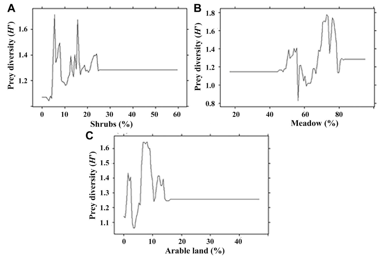
After the most relevant variables had been identified, the next step was to attempt to understand how the response variable changes based on these variables. To do this we used partial dependence plots (PDPs). For example, consider the "shrubs (%)" variable from Fig. 2, the PDP plot below displays the average change in predicted prey diversity (H′) as we vary shrubs (%) while holding all other variables constant. This is done by holding all variables constant for each observation in our training data set but then we apply the unique values of "shrubs (%)" for each observation. We then averaged the prey diversity across all the observations. This PDP illustrates how the predicted prey diversity increases as the shrubs (%) increases. The stable lines are those values of the independent variables for which there are no data on the dependent variable. It can be removed, but usually at the same works (Domahidi et al., 2019) it is used, and we also decided to use.
The first model contained the share of Common Vole in the model species diet as response variable. The share of different land cover classes (shrubs, meadow, arable land, forest), coefficient of habitat heterogeneity (K) and Common Vole abundance in the hunting territory were used as quantitative predictors. Locations that did not fit this classification were used as a separate predictor called "Other". The presence/absence of ditches and roads, as well as bird species were used as qualitative predictors.
The second model contained the share of Root Vole in the model species diet as response variable. The share of different land cover classes (shrubs, meadow, arable land, forest), coefficient of habitat heterogeneity (K) and Root Vole abundance in the hunting territory were used as quantitative predictors. Locations that did not fit this classification were used as a separate predictor called "Other". The presence/absence of ditches and roads, as well as bird species were used as qualitative predictors.
The third model contained the Shannon–Wiener Index as response variable. The share of different land cover classes (shrubs, meadow, arable land, forest), coefficient of habitat heterogeneity (K) and the abundance of the two main types of prey on them and the species of bird were used as predictors. Locations that did not fit this classification were used as a separate predictor called "Other". The presence/absence of ditches and roads, as well as bird species were used as qualitative predictors.
After the most relevant variables have been identified, the next step is to attempt to understand how the response variable changes based on these variables. For this we can use partial dependence plots (De'Ath, 2007; Elith et al., 2008).
A total of 7628 individuals were identified from prey remains. The Long-eared Owl diet composition contained prey items of all vertebrate classes, insects and mollusks (Table 1). Small mammals represented 96.9% of the diet. Root Vole (43.7%) and Common Vole (42.1%) were the main prey. The percentages of other vertebrates, as well as insects, did not exceed 2% (Table 1).
| Prey category | Long-eared Owl | Short-eared Owl | Falco tinnunculus | |||||
| n | % | n | % | n | % | |||
| Mammals | 3442 | 96.9 | 534 | 99.2 | 2103 | 59.5 | ||
| Microtus arvalis | 1495 | 42.1 | 410 | 76.2 | 682 | 19.3 | ||
| Microtus oeconomus | 1552 | 43.7 | 112 | 20.8 | 722 | 20.4 | ||
| Other mammals | 395 | 11.1 | 12 | 2.2 | 699 | 19.8 | ||
| Aves | 34 | 1.0 | – | 0.0 | 42 | 1.2 | ||
| Reptilia | 3 | 0.1 | 1 | 0.2 | 36 | 1.0 | ||
| Amphibia | 7 | 0.2 | – | 0.0 | 5 | 0.14 | ||
| Pisces | 39 | 1.1 | – | 0.0 | – | – | ||
| Insecta | 28 | 0.8 | 3 | 0.6 | 1348 | 38.1 | ||
| Mollusca | 1 | 0.03 | – | 0.0 | 2 | 0.06 | ||
| Total | 3554 | 100.0 | 538 | 100.0 | 3536 | 100.0 | ||
 DownLoad:
CSV
DownLoad:
CSV
Small mammals are the basis of the Short-eared Owl diet (99.2%). The main prey species were Common Vole (76.2%) and Root Vole (20.8%). We also noted representatives of the reptile class (Reptilia) (0.2%), as well as insects (0.6%) in the diet of the Short-eared Owl (Table 1).
The main prey in the Common Kestrel diet were small mammals; however, the percentage was lower than in the diet of the two owl species (59.5%). The Common Vole (19.3%) and Root Vole (20.4%) were dominant species. The second place in the diet of the birds was occupied by insects (38.1%). The percentage of other classes of prey was less than 2%. Thus, the two species of Microtus voles play a significant role in the diet of the studied birds.
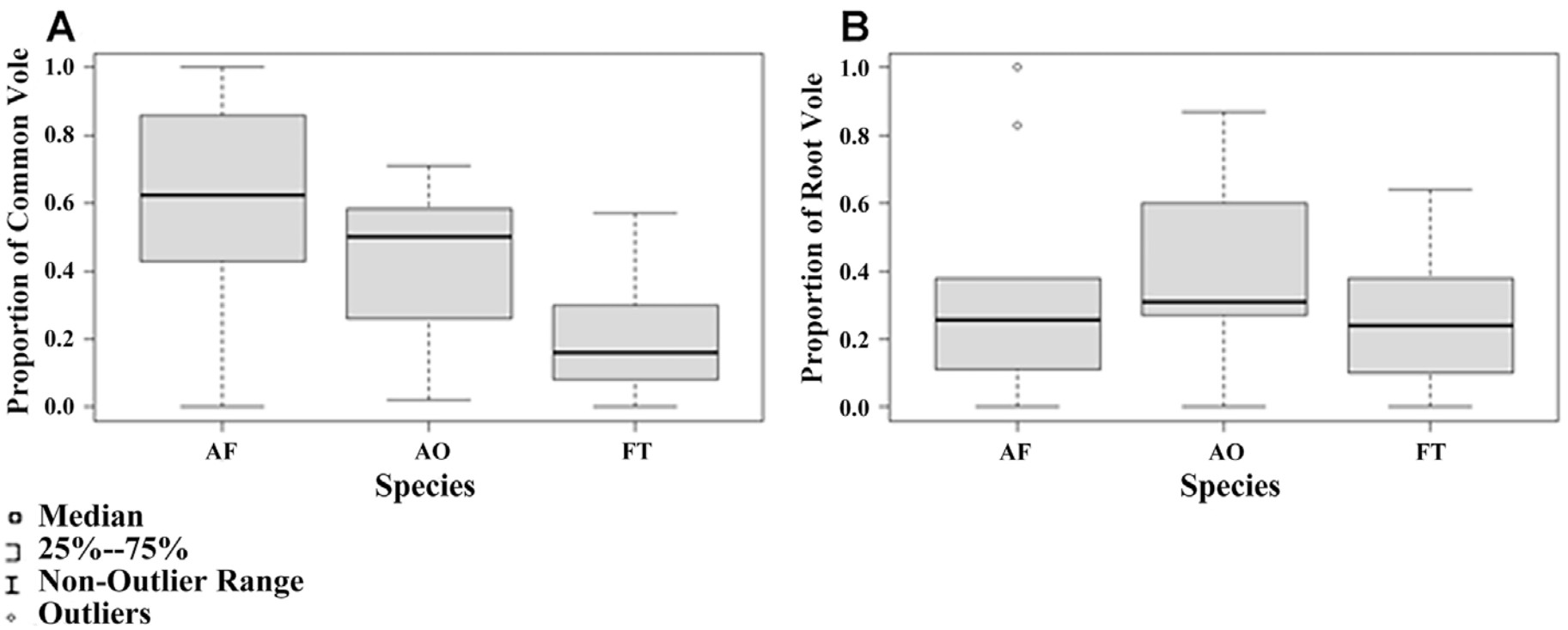
Proportions of the two vole species in the diets of the studied predators differed (Table 1; Fig. 3). The proportion of Common Vole was highest in the Short-eared Owl diet and lowest in the Common Kestrel diet. The proportion of Root Vole was highest in the Long-eared Owl diet (Fig. 3). However, the species preferences of the predators had no significant effect as a presence of two voles' species in the diets (Table 2).
| Predictors | Dependent variables | ||
| Microtus arvalis | Microtus oeconomus | Prey diversity (H′) | |
| Shrubs | 18.8 | 23.2 | 20.1 |
| Meadow | 18.0 | 17.7 | 18.8 |
| Habitat heterogeneity (K) | 15.4 | 13.5 | 12.4 |
| Arable land | 14.6 | 16.2 | 14.3 |
| Village | 10.5 | 12.3 | 7.7 |
| Species* | 9.2 | 3.7 | 8.8 |
| Forest | 5.5 | 10.1 | 8.1 |
| Microtus arvalis abundance | 5.3 | – | 1.2 |
| M.oeconomus abundance | – | 1.0 | 5.1 |
| Water | 2.4 | 1.7 | 2.4 |
| Other | 0.1 | 0.4 | 0.9 |
| Road | 0.1 | 0.1 | 0.2 |
| Predictors which made the greatest contribution to the model predictions are highlighted in bold. * – species of birds: Long-eared Owl, Short-eared Owl and Common Kestrel. | |||
DownLoad:
CSV
Moreover, the abundance of both main prey species of voles in the hunting territories did not significantly affect their presence in the diet of owls and kestrel (Table 2). The influence of voles' abundance was lower than other factors.
The species diversity and the number of rare species in the diet of model bird species were most influenced by the presence of shrubs, meadows and arable land on hunting areas (Fig. 2). The highest species diversity in the diet of birds was noted in the presence of 5% of shrubs in the hunting territories (Fig. 2). The second significant predictor was the presence of 65% of meadows where the greatest species diversity of prey was noted (Fig. 2). In addition, the highest prey diversity was noted when there was 8% of arable land areas on the hunting territories of birds. The fourth important predictor was the habitat heterogeneity (Table 2), which contributed 12.4% to the model predictions.
Despite the fact that the highest prey diversity was found in the diet of the Common Kestrel, the "species" predictor did not have a significant effect (Table 2).
According to the modeling results (Table 2), the most significant predictors influencing the diet composition and the proportion of the two vole species in it were the size of the shrubs area, the size of the meadow area, the habitat heterogeneity and the size of the arable lands on the hunting territories.
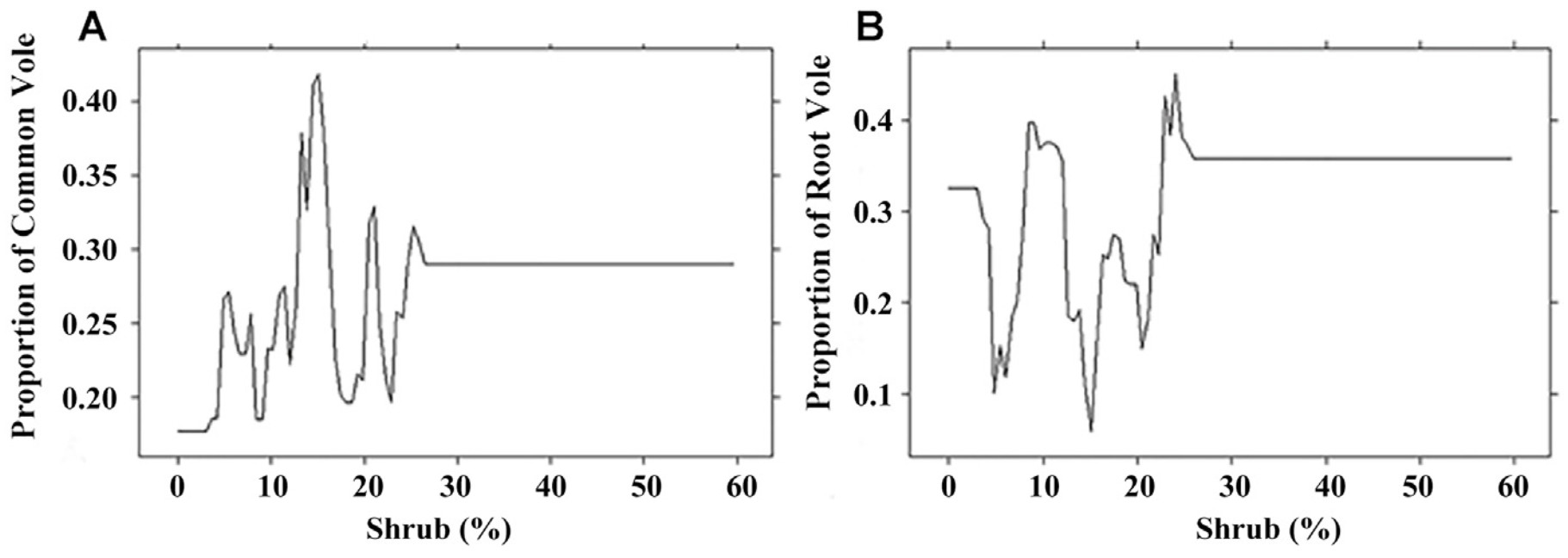
The strongest predictor influencing the presence of the two main prey species in the diet of birds of prey was the size of shrubs area in the hunting territory. Voles were found in the diet in the territories where the area of shrubs did not exceed 25% (Fig. 4). The largest rate of the Common Vole in the diet of the predators was noted in territories where the shrub cover was 15%, for the Root Vole 25%.
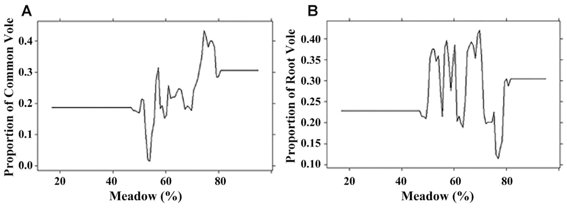
The area of meadows was the second important predictor (Table 2). Voles were found in prey on hunting areas where meadows occupied from 45% to 82% of the territory (Fig. 5). Largest rates of the Common Vole and the Root Vole in the diet of the predators were found in the territories where meadows covered 75% and 70% of the land area, respectively.
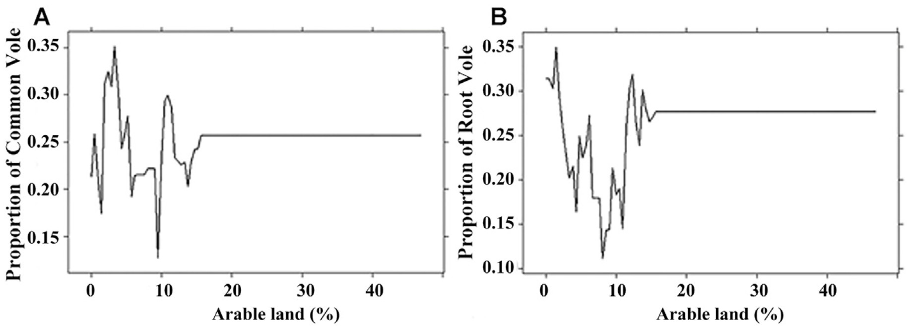
The area of the arable land was the third most important factor. Voles were found in the diet where the arable land covered less than 15% of the hunting territory (Fig. 6). The largest proportions of Common Vole and Root Vole in the diet were recorded where the share of arable land was 5% and 3% respectively.
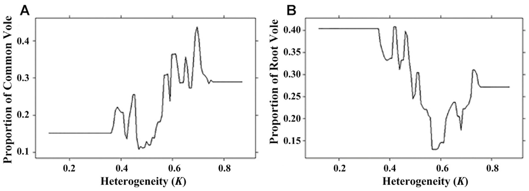
The heterogeneity of hunting territories (K) was the third important factor influencing the composition of the diets of birds of prey. At the same time, the lowest proportions of both vole species were observed at territories with both high and low index of habitat heterogeneity. The Common Vole was preyed in territories with a heterogeneity range of 0.35–0.75; for the Root Vole 0.37–0.77 (Fig. 7). The largest rate of the Common Vole in diet was noted at hunting territories with a high index of heterogeneity (0.7). Root Vole is maximally represented in the raptors' diet at hunting territories with a low heterogeneity index (0.45) (Fig. 7).
The Common Vole and Root Vole were also noted as the main prey species for the Common Kestrel, Long-eared and Short-eared Owls in the study area in previous studies (Sharikov et al., 2016; Buslakov and Sharikov, 2018). The Microtus voles are the main prey for both owl species and kestrel in general (Schnurre and Creuzburg, 1971–1974; Schmidt, 1975; Sharikov et al., 2016). Traditionally it is considered that the abundance of voles is the main factor determining their presence in the diet of birds of prey (Pyke, 1984; Korpimäki, 1985, 1992; Korpimäki and Norrdahl, 1991; Davorin, 2009). The model species are predators that demonstrate cyclical fluctuations associated with annual changes of the main prey abundance (Cramp, 1985; Tome, 2009; Volkov et al., 2009). Interannual fluctuations of Microtus voles' abundance impact the diet composition of most medium-sized birds of prey (Village, 1981; Korpimäki and Norrdahl, 1991; Tome, 2003). However, natural habitats with a high abundance of prey are not necessarily the best for hunting. The availability of prey in certain habitats can be affected by various factors (Sonerud, 1986; Aschwanden et al., 2005). The habitat features of the hunting territory play a significant role and this assumption is also confirmed by our study.
The abundance of the Common Vole and Root Vole was not a significant predictor determining the high proportion of these species in the diet of avian predators. In contrast, the habitat structure of hunting territories carries an important value. The highest rate of the main prey species was found in the diet of birds that hunted in areas with a large proportion of open spaces and low shrubs. Thus, we confirmed that the relative importance of habitat structure versus prey abundance. It opens a new way of thinking about the optimal foraging theory because this is contrary to the provision of most important role of prey abundance.
The highest proportion of the Common Vole was noted in the diet of birds that hunted in areas with high percentage of open spaces and low percentage of shrubs. In contrast, the highest rate of the Root Vole was recorded in territories with higher percentage of shrubs and lower percentage of open spaces with lower habitat heterogeneity. This difference could be explained by different habitat preferences of the Common Vole and the Root Vole. The Root Vole prefers more bushy areas and often becomes a prey of Long-eared Owls. According to previous studies, preferred foraging habitats for our model species include woodland and agricultural edges, grass fields, meadows and bogs (Cramp, 1985; Galeotti et al., 1997). Most of the studies are devoted to habitat selection of Long-eared Owls. In Czech Republic Long-eared Owls used the territories with 62.4% of open areas, 17.2% of coniferous forests and 4.1% of deciduous forests (Ševčík et al., 2021). Data on the habitat selection of Long-eared Owls have been reported from several European regions including the Mediterranean basin where the dominant land cover type was dry arable land or mosaics of several rural land-use types such as cultivations, irrigated crops, tree plantations, orchards, vineyards and rural settlements (Martínez and Zuberogoitia, 2004; Leader et al., 2008; Bartolommei et al., 2012). The importance of open area such as grassland is interestingly explained by George and Johnson (2021). In the Napa Valley grassland is the most abundant uncultivated habitat within range of the Barn Owls' nests, and they offer high densities of rodents. Therefore, having more of this habitat near the nest box may allow Barn Owls to meet higher energetic demands of chicks by reducing the commute and search time for prey (George and Johnson, 2021). The high importance of shrubs in the hunting area can be explained by using capture time to assess the timing of mouse activity: mice in habitats with minimal shrub cover were captured by raptors 1.7 h earlier than mice in habitats with abundant shrub cover (Connolly and Orrock, 2018).
Consequently, the proportion of the main prey species in the diet of birds depends on the structure of the hunting territory. A positive relationship between the area of open spaces in hunting territories and the share of Microtus voles in the diet of birds of prey was shown in previous studies. For example, it has been found that the proportion of Microtus voles in the diet of Long-eared Owls was positively associated with an increase in the proportion of meadows with low vegetation. The proportion of mice was negatively associated with this habitat (Romanowski and Zmihorski, 2008). Similar results were obtained in a study of changes in the Barn Owl diet composition (Milchev, 2015; Szép et al., 2017).
In addition, the species diversity of prey and the number of rare species in the diet of birds of prey is associated with the heterogeneity of hunting territories (Szép et al., 2017). A positive correlation was shown between the diversity of small mammals in the diet of Barn Owls and the complexity of the landscape of their hunting territories (Szép et al., 2017). For our species the higher prey diversity in the diet was found on territories with low habitat heterogeneity. In general, the habitat heterogeneity was the fourth important predictor affecting the diversity of prey in the diet of the studied bird species. Thus, the prey diversity is not always associated with mosaic habitats and may be higher on homogeneous territories. In addition, the species-specific preferences of birds also did not have a strong effect on the diversity of prey in their diets.
Thus, our results suggest that habitat characteristics are a main factor determining prey choices. Perhaps this is due to prey accessibility and availability in different types of hunting territory. Prey abundance in the hunting territory is a less important factor. Thus, the model species are targeted to hunt in territories with certain ratio of habitat elements than territories with a high abundance of the main prey species, which leads to a greater diet diversity.
Conceptualization: T.K. & A.S.; Data curation: T.K.; Methodology: T.M.; Writing – original draft: T.K.; Writing – review & editing: A.S. & S.V. All authors read and approved the final manuscript.
The study was conducted according to the guidelines of the Declaration of Helsinki, and approved by the Institutional Review Board of Moscow Pedagogical State University, Institute of Biology and Chemistry, Department of Zoology and Ecology (protocol code No. 1, date of approval: 31.08.2021).
The authors declare that they have no competing interests.
We are grateful to O.S. Grinchenko, director of Crane's Homeland Reserve for the opportunity to conduct the study on this place. We are grateful to K.V. Makarov for his help with insects' identification. We also thank E.M. Shishkina and V.V. Buslakov for their help in collecting and analysing pellets and the students and postgraduates of Moscow Pedagogical State University who took part in the field research.
|
Breiman, L., Friedman, J.H., Olshen, R.A., Stone, C.G., 1984. Classification and Regression Trees. Wadsworth International, New York.
|
|
Buslakov, V.V., Sharikov, A.V., 2018. Diet diversity of the Common Kestrel Falco tinnunculus in the northern Moscow region and its interannual variability. Russ. Ornithol. J. 27, 2992-2993.
|
|
Cramp, S., 1985. Handbook of the Birds of Europe, the Middle East and North Africa.
Oxford University Press, Oxford.
|
|
Galeotti, P., Tavecchia, G., Bonetti, A., 1997. Home-range and habitat use of Long-eared Owls in open farmland (Po plain, northern Italy), in relation to prey availability. J. Wildl. Res. 22, 137-145.
|
|
Grinchenko, O.S., Sviridova, T.V., Kontorshchikov, V.V., 2020. Long-term dynamics of ecosystems in the northern Moscow region (substantiation of the creation of a natural park "Crane land"). Ecosyst. Ecol. Dynam. 4, 104-137.
|
|
Gromov, I.M., Yerbaeva, M.A., 1995. Mammalian Fauna of Russia and Adjacent Territories (St. Petersburg, Russia).
|
|
Kodzhabashev, N.D., Dipchikova, S.M., Teofilova, T.M., 2020. Landscape structure impacts the small mammals as prey of two wintering groups of Long-eared Owls (Asio otus L.) from the region of Silistra (NE Bulgaria). Ecol. Balkanica 3, 129-138.
|
|
Korpimäki, E., 1985. Diet of the Kestrel Falco tinnunculus in the breeding season. Ornis Fennica 62, 130-137.
|
|
Korpimäki, E., 1981. On the ecology and biology of Tengmalm's Owl (Aegolius funereus) in southern Ostrobothnia and Soumenselka, western Finland. Acta Univ. Oul. A. Sci. Rer. Nat. 118, 1-84.
|
|
Mikkola, H., 1983. Owls of Europe. T. and A.D. Poyser, Calton, UK.
|
|
Naumov, R.L., 1963. Organization and Methods of Recording Birds and Harmful Rodents (Moscow, Russia).
|
|
R Core Team, 2012. R: A Language and Environment for Statistical Computing. R Foundation for Statistical Computing, Vienna.
|
|
Romanowski, J., Zmihorski, M., 2008. Effect of season, weather and habitat on diet variation of a feeding-specialist: a case study of the Long-eared Owl, Asio otus in Central Poland. Folia Zool. 57, 411-419.
|
|
Schmidt Е., 1975. Die Ernahrung der Waldohreule (Asio otus) in Europa. Aquila 80-81, 221-238.
|
|
Schnurre, O., Creuzburg, V., 1971-1974. Zur Ernährung der Waldohreule (Asio otus) im Berliner Raum. Aquila 3, 742-747.
|
|
Selçuk, A.Y., Bankoğlu, K., Kefelioğlu, H., 2017. Comparison of winter diet of long-eared owls Asio otus (L., 1758) and short-eared owls Asio flammeus (Pontoppidan, 1763) (Aves: strigidae) in northern Turkey. Acta Zool. Bulg. 69, 345-348.
|
|
Shannon, C.E., Weaver, W., 1949. The Mathematical Theory of Communication. University of Illinois Press, Urbana, IL.
|
|
Sharikov, A.V., Makarova, T.V., 2014. Weather conditions explain variation in the diet of Long-eared Owl at winter roost in central part of European Russia. Ornis Fennica 91, 100-107.
|
|
Sharikov, A.V., Shishkina, E.M., Volkov, S.V., 2016. Diet composition of owls in the North of Moscow Region. Bull. Cranes Homeland 3, 14-21.
|
|
Sharikov, A.V., Volkov, S.V., Sviridova, T.V., Buslakov, V.V., 2019. Impact of trophic and weather-climatic factors on the numbers dynamics of vole-eating birds of prey in their breeding habitats. Zool. J. 98, 203-213.
|
|
Tome, D., 2009. Changes in the diet of Long-eared Owl Asio otus: seasonal patterns of dependence on vole abundance. Ardeola 56, 49-56.
|
|
Tome, D., 2003. Functional response of the Long-eared Owl (Asio otus) to changing prey numbers: a 20-year study. Ornis fennica 80, 63-70.
|
|
Village, A., 1981. The diet and breeding of Long-eared owls in relation to vole number. Bird study 28, 215-224.
|
|
Vinogradov, B.V., 1998. Fundamentals of Landscape Ecology. GEOS, Moscow, Russia.
|
|
Volkov, S.V., Sharikov, A.V., Basova, V.B., Grinchenko, O.S., 2009. The influence of the abundance of small mammals on the selection of habitats and population dynamics of the Long-eared (Asio otus) and Short-eared (Asio flammeus) Owls. Zool. J. 88, 1248-1257.
|
Figures(7) / Tables(2)


| Prey category | Long-eared Owl | Short-eared Owl | Falco tinnunculus | |||||
| n | % | n | % | n | % | |||
| Mammals | 3442 | 96.9 | 534 | 99.2 | 2103 | 59.5 | ||
| Microtus arvalis | 1495 | 42.1 | 410 | 76.2 | 682 | 19.3 | ||
| Microtus oeconomus | 1552 | 43.7 | 112 | 20.8 | 722 | 20.4 | ||
| Other mammals | 395 | 11.1 | 12 | 2.2 | 699 | 19.8 | ||
| Aves | 34 | 1.0 | – | 0.0 | 42 | 1.2 | ||
| Reptilia | 3 | 0.1 | 1 | 0.2 | 36 | 1.0 | ||
| Amphibia | 7 | 0.2 | – | 0.0 | 5 | 0.14 | ||
| Pisces | 39 | 1.1 | – | 0.0 | – | – | ||
| Insecta | 28 | 0.8 | 3 | 0.6 | 1348 | 38.1 | ||
| Mollusca | 1 | 0.03 | – | 0.0 | 2 | 0.06 | ||
| Total | 3554 | 100.0 | 538 | 100.0 | 3536 | 100.0 | ||
DownLoad:
CSV
| Predictors | Dependent variables | ||
| Microtus arvalis | Microtus oeconomus | Prey diversity (H′) | |
| Shrubs | 18.8 | 23.2 | 20.1 |
| Meadow | 18.0 | 17.7 | 18.8 |
| Habitat heterogeneity (K) | 15.4 | 13.5 | 12.4 |
| Arable land | 14.6 | 16.2 | 14.3 |
| Village | 10.5 | 12.3 | 7.7 |
| Species* | 9.2 | 3.7 | 8.8 |
| Forest | 5.5 | 10.1 | 8.1 |
| Microtus arvalis abundance | 5.3 | – | 1.2 |
| M.oeconomus abundance | – | 1.0 | 5.1 |
| Water | 2.4 | 1.7 | 2.4 |
| Other | 0.1 | 0.4 | 0.9 |
| Road | 0.1 | 0.1 | 0.2 |
| Predictors which made the greatest contribution to the model predictions are highlighted in bold. * – species of birds: Long-eared Owl, Short-eared Owl and Common Kestrel. | |||
DownLoad:
CSV
 Email Alerts
 RSS Feeds