Lubna ALI, Noor-un-nisa, Syed Shahid SHAUKAT, Rafia Rehana GHAZI. 2011: Sex and age classes of prey items (rats/mice) in the diet of the Barn Owl (Tyto alba) in Sindh, Pakistan. Avian Research, 2(2): 79-86. DOI: 10.5122/cbirds.2011.0012
Citation:
Lubna ALI, Noor-un-nisa, Syed Shahid SHAUKAT, Rafia Rehana GHAZI. 2011: Sex and age classes of prey items (rats/mice) in the diet of the Barn Owl (Tyto alba) in Sindh, Pakistan. Avian Research, 2(2): 79-86. DOI: 10.5122/cbirds.2011.0012
Lubna ALI, Noor-un-nisa, Syed Shahid SHAUKAT, Rafia Rehana GHAZI. 2011: Sex and age classes of prey items (rats/mice) in the diet of the Barn Owl (Tyto alba) in Sindh, Pakistan. Avian Research, 2(2): 79-86. DOI: 10.5122/cbirds.2011.0012
Citation:
Lubna ALI, Noor-un-nisa, Syed Shahid SHAUKAT, Rafia Rehana GHAZI. 2011: Sex and age classes of prey items (rats/mice) in the diet of the Barn Owl (Tyto alba) in Sindh, Pakistan. Avian Research, 2(2): 79-86. DOI: 10.5122/cbirds.2011.0012
Vertebrate Pest Control Institute, Southern-zone Agricultural Research Centre, Pakistan Agricultural Research Council, P. O. Box-8401 Karachi University Campus, Karachi-75270, Pakistan
2.
Institute of Environmental Studies, University of Karachi, Karachi-75270, Pakistan
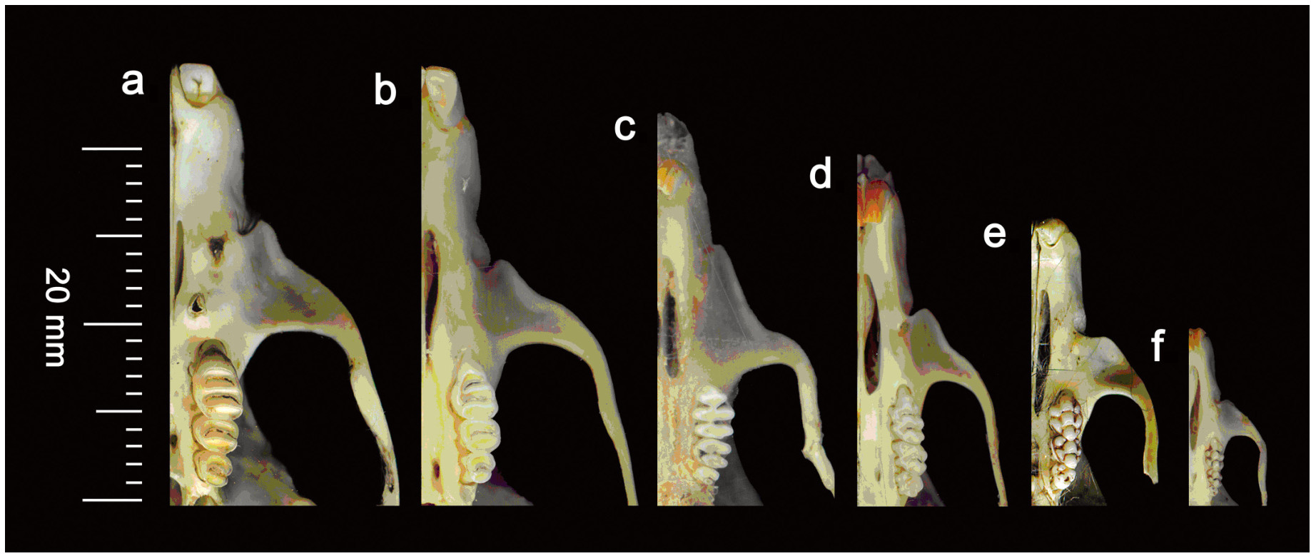
Barn Owl (Tyto alba) pellets were collected from nine locations and two districts of Sindh, Pakistan and 937 prey items were recovered from 619 pellets. Rats/mice (59.6%) were the most dominant food items consumed by the Barn Owl. Shrews (22.3%), bats (1.3%), birds (12.0%), insects (1.3%), frogs (2.2%) and plant materials (1.3%) were found in their diet as well. Study of the pelvic girdle bones of rats/mice, used only for sexing, proved to be a useful device in population dynamics. In the pelvic bone, pelvic symphysis is found only in female rats/mice developed as a result of sex hormones that occur during gestation. Among the diet of rats/mice, males were found to be significantly dominant. Tooth wear patterns on the occlusal surfaces of molariform teeth of the rats/mice were found to provide an effective criterion for establishing age classes of rats/mice. In the present study, adult rats/mice were found to be dominant over sub-adults and old adults. ANOVA showed significant differences in the number of rats/mice and shrews (prey items) and the other prey items/plant materials in the diet of Barn Owls in the district Thatta and district Karachi. Chi-square test disclosed non-significant differences in age and sex categories.
The primary driver of the global decline in biodiversity is habitat loss and fragmentation, caused by anthropogenic pressure on natural ecosystems. Urbanization is arguably the most damaging, persistent and rapid form of anthropogenic pressure (Morneau et al., 1999; Park and Lee, 2000; Porter et al., 2001; Clergeau et al., 2006). Although studies in London have demonstrated that the changes of urban building structures and vegetation affect the abundance of urban House Sparrows (Passer domesticus) (Peach and Vincent, 2006; Chamberlain et al., 2007), there is little information about the effect of urbanization on the abundance of the bird species closely linked to human environments in a rapidly developing country such as China.
The Tree Sparrow (Passer montanus) is one of the most common birds found in a variety of environments along urban gradients in China (Ruan and Zheng, 1991; Pan and Zheng, 2003), which makes it a suitable model species to study the effects of urbanization on birds closely linked to human environments. They nest in hollows of buildings and eat small seeds (Ruan and Zheng, 1991); therefore, the distribution of this species is closely related to human environments. China's capital, Beijing, provides an example of a city with rapid urbanization during the last 20 years. The construction of new high-rise buildings have resulted in reduction of vegetation and the demolition of old buildings, reducing the food and habitat of the Tree Sparrow (Zhang et al., 2008). The abundance and distribution of Tree Sparrows are likely to be affected by habitat and food losses in Beijing. For these reasons, the objective of this study is to test whether the degree of urbanization affects the abundance of Tree Sparrows and what environmental factors impact the distribution pattern of this species.
Scale is an important aspect involved in most ecological problems (Levin, 1992; Willis and Whittaker, 2002). Urban planning is also a multi-scale process encompassing both local scale design such as the structure of residential areas and landscape scale design such as the distribution of buildings and vegetation (Savard et al., 2000; Hostetler and Kim, 2003; Melles et al., 2003). Some earlier studies used a theory of island biogeography to predict the relationship between urban bird distribution and characteristics of native habitat patches (e.g., a large park) such as patch size and the degree of isolation from other areas of habitat (Tilghman, 1987; Diamond, 1988; Soulé et al., 1988). Since the presence of birds was expected to vary with land use pattern and with the overall composition of the landscape in a complex landscape mosaic (Trzcinski et al., 1999; Austen et al., 2001; Fahrig, 2001), the biogeography theory was not sufficient for many urban scenarios. More and more recent studies have been carried out based on spatial-structuring theories in which local-scale and landscape-scale habitat features surrounding the habitats were combined to predict the habitat factors affecting urban bird distributions (Bolger et al., 1997; Rottenborn, 1999; Odell and Knight, 2001; Melles et al., 2003; Hostetler and Kim, 2003; Hiroshi et al., 2005). Although our previous work has discussed the factors affecting the distribution of Tree Sparrows in Beijing, the habitat variables in that study were only on a local scale (Zhang et al., 2008). Therefore, in this study we hope to discuss this question of multiple scales based on spatial-structuring theories in order to predict the factors affecting the distribution of Tree Sparrows more comprehensively.
Methods
Study area and sampling design
Beijing is situated in the North China Plain. The urban area spreads out in bands of six concentric ring roads. The climate of the city consists of a hot, humid summer and a cold, windy and dry winter. The average daytime high temperature in January is 1.6℃, while in July it is 30.8℃. Annual precipitation is around 580 mm.
Eight land use types were selected for analysis, i.e., suburban (SU), low building residential areas (LB), high-rise building residential areas (HB), brick bungalow areas (BB), commercial centers (CC), parks (PA), university campuses (UC) and main roads (MR). In these types, high-rise building residential areas, commercial centers and main roads are three urbanized land use types. With high-rise buildings we mean buildings higher than six floors, most of which were constructed after the 1990s; low buildings means the buildings lower than six floors, mostly constructed before the 1990s. The area within the fifth circle of Beijing was divided into four parts using Tiananmen Square as the center, Chang An Street as the X-axis and the meridian of the Forbidden City (the Dragon line) as the Y-axis. In each part, study sites were selected randomly and, in total, five to ten study sites were selected in the four parts for each land use type (Table 1).
Table
1.
Land use types and their study sites
Land use types
Study sites
Suburban area
Xidian and Fangjia villages of Gaobeidian, Xiaoying Village of Daxing District, Babaoshan, and Nanshuitouzhuang Nanli
Park
Zizhuyuan Park, Yuyuantan Park, Botanical Garden, Yuanmingyuan Park, Haidian Park, the Summer Palace, Tiantan Park, and Ditan Park
University campus
Peking University, Beijing Normal University, Renmin University of China, Beijing Jiaotong University, Beijing Institute of Technology, Beijing Foreign Studies University, Capital Normal University
Low building residential area
Weigongcun Community, Guanyuan, Dongguantou Street, Canjiakou Community
High-rise building residential area
Tiantongyun residential quarter, Weibohao Community, Lianhua Community, and Tuanjie Community
Commercial center
Xidan, Chengxiang Trade Center, Zhongguancun, Haidian Books Market, Wangfujing Street, and Finance Avenue
Main road
Chegongzhuang Avenue, Gulou Avenue, Wukesong, Huayuanqiao, Zhongguancun Avenue, Qinghua West Avenue, and Weigongcun Road
Brick bungalow area
Dongdan, Dongguantou Street, West of Lianhua community, and Zhongshan Park
We used an "urbanization score" (Liker et al., 2008) to quantify the degree of urbanization of the study sites and their surroundings. The occurrence of three important land cover types for birds, i.e., buildings, paved roads and vegetated areas were scored. One 1 km × 1 km area around each capture site was selected from high-resolution digital aerial photographs. Each 1 km2 area was divided into 100 cells (using a 10 × 10 grid with their scores), indicating levels of building cover (0, absent; 1, < 50%; 2, > 50%), the presence of roads (0, absent; 1, present) and vegetation cover (0, absent; 1, < 50%; 2, > 50%) for each cell. From these cell scores the following summary statistics for all seven capture sites were calculated: a mean building density score (potential range 0–2), the number of cells with high-rise building density (> 50% cover; range 0–100), the number of cells with roads (range 0–100), a mean vegetation density score (range 0–2) and the number of cells with high vegetation density (> 50% cover; range 0–100). The PC1 score of a principal components analysis of these five summary scores was taken as the overall "urbanization score" for each site. Principal components analysis extracted only one component, accounting for 95% of the total variance. From the loading of the original variables, higher urbanization scores can be interpreted as reduced vegetation density and increased building and road densities.
Habitat variables
Ten habitat variables at the local scale (a circle with a 50 m radius around Tree Sparrow-present points) and three landscape factors at three scales (circles with a radius of 200, 400 or 600 m around Tree Sparrow-present points) were selected to investigate the major factors affecting the distribution of Tree Sparrows (Table 2). At a local scale, the habitat factors include areas of high-rise buildings, pavement and weeds, number of conifer and broad-leaved trees, areas of low buildings, number of air conditioners (major nesting sites of urban Tree Sparrows), distance to main roads, number of pedestrians and vehicle flux. At the landscape scale, areas of high-rise buildings, reflecting a degree of modernization, low buildings and vegetation were selected.
Table
2.
Definitions of habitat variables on local and landscape scales
Scales
Variables
Descriptions of variables
50 m
Area of high-rise buildings
Buildings higher than six floors
Area of pavements
Paved landscape including bitumen or cement bricks
Area of weeds
Natural lawn comprising weeds which provide food resources for Tree Sparrows
Number of broad-leaved trees
Broad-leaved trees can provide shelters for Tree Sparrows
Number of conifer trees
Observations indicated conifers may provide alternate roosting sites for Tree Sparrows during winter
Area of low buildings
Low buildings include brick bungalows, ancient buildings and the buildings lower than six floors. These buildings provide nest sites for Tree Sparrows
Number of air conditioners
Air conditioners installed on the exterior of buildings can be used as nest sites by Tree Sparrows
Distance to main roads
Roads comprising of more than three lanes of traffic
Number of pedestrians
Pedestrians passing the study site over a 10-min duration
Vehicle flux
Moving cars, motorbikes, trucks etc. passing the study sites over a 10-min duration
200 m, 400 m, 600 m
High-rise buildings (HB)
Area percentage of buildings higher than six floors in a circle area around the Tree Sparrow present points
Low buildings (LB)
Area percentage of buildings lower than six floors in a circle area around the Tree Sparrow present points
Vegetation (VE)
Area percentage of vegetation in a circle area around the Tree Sparrow present points
From January to August 2005, we surveyed the number of Tree Sparrows and local-scale habitat variables during the wintering period (January to March) and the breeding period (April to August). At each study site, we walked along 2–3 roads which traverse the study sites, recording the number of Tree Sparrows and the corresponding GPS coordinates of their locations, as used points for a one-hour time period. Randomly selected locations in all study sites were used as control points where their GPS coordinates were recorded. Following each avian survey we assessed local-scale habitat variables in areas using a circle with a 50 m radius, with each used and control point as a center. In total, we surveyed 239 used points and 118 control points in the winter and 226 used points and 126 control points in the breeding period. Areas and distances were measured with the GPS. Using satellite images acquired from Google Earth Web, we digitized the landscape variables for each used and control point using ArcGis and ArcView 3.2 to identify low building areas, high-rise building areas and vegetation areas. Low buildings and high-rise buildings were determined by local surveys according to the corresponding coordinates on the satellite images where they were difficult to be distinguished on the images. We created circles with a radius of 200, 400 or 600 m around each of the used and control points, after which we measured the areas of the three landscape variables using Spatial Analysist, the X-Tool and Geoprocessing extensions of ArcView3.2.
Data analysis
We used one-way ANOVA to compare the number of Tree Sparrows of different land use types and Tukey's Honestly Significant Difference (HSD) post hoc tests to conduct pairwise comparisons between land use types. The average number of Tree Sparrows (recorded within one hour in each study site) and the urbanization scores of all study sites for one land use type was used as the score for the number of Tree Sparrows and urbanization for each land use type. To analyze whether the number of Tree Sparrows is directly related to the degree of urbanization, we investigated the correlation between the score of the number of Tree Sparrows and the urbanization scores of eight land use types, using Pearson correlation analysis.
We used stepwise elimination logistic regression to analyze the appropriate scales and key factors affecting the distribution of Tree Sparrows. Prior to the logistic regression, we first selected the habitat variables with significant differences between used and control sites using independent t-tests or the Mann-Whitney U-test. Using these variables, we created a 50 m scale model and three models integrating this scale model with those of a 200, 400 and 600 m scale respectively. The best fitting model was selected using Akaike's information criterion (AIC). All data were standardized to a normal distribution before logistic regression. The data analyses were performed with SPSS 11.0.
Results
Correlation between number of Tree Sparrows and degree of urbanization
The number of Tree Sparrows differed significantly among land use types (wintering period: one-way ANOVA, df = 7, F = 25.23, p < 0.001; breeding period: df = 7, F = 19.97, p < 0.001). The number of Tree Sparrows was highest in parks and lowest in commercial centers. Pairwise comparisons between land use types showed that the number of birds in commercial centers, high-rise residential areas and main roads were significantly lower than in parks, suburban areas and university campuses, both in the wintering period (Turkey's HSD test, CC vs. PA, CC vs. SU, CC vs. UC, HB vs. PA, HB vs. UC, MR vs. PA, MR vs. UC, MR vs. SU, p < 0.001; HB vs. SU, p = 0.046) and in the breeding period (Turkey's HSD test, CC vs. PA, CC vs. SU, CC vs. UC, HB vs. PA, HB vs. UC, MR vs. PA, MR vs. UC, MR vs. SU, p < 0.001; HB vs. SU, p = 0.013) (Fig. 1).
Figure
1.
Number of Tree Sparrows in eight land use types
The number of Tree Sparrows was negatively correlated with urbanization scores in both the wintering and breeding periods (wintering period: n = 8, r = –0.832, p = 0.010; breeding period: n = 8, r = –0.863, p = 0.006) (Fig. 2).
Figure
2.
Relationship between number of Tree Sparrows in different land use types and capture site urbanization scores in breeding period (a) and wintering period (b)
Habitat factors affecting distribution of Tree Sparrows
Within four models of the wintering period, the AIC was lowest at the 50 m × 200 m scale, suggesting this scale to be the most suitable for predicting environmental factors affecting Tree Sparrow abundance. The number of conifer trees and pedestrians are the two major factors on the 50 m scale, while areas of high-rise buildings and vegetation were the predominant factors on the 200 m scale (Table 3). In comparison to used points, the number of conifer trees and area percentage of vegetation was significantly lower in control points (independent t-test p < 0.001), indicating these two factors are advantageous in the distribution of Tree Sparrows. In contrast, the number of pedestrians and area percentage of high-rise buildings in used points were significantly lower compared to control points (Independent t-test p < 0.001). This indicates that these two factors have a negative effect on Tree Sparrow abundance (Table 4).
Table
3.
Parameters of obtained equations of logistic regressions on different scales in winter and summer
During the summer, the 50 m × 400 m model resulted in a regression equation with the lowest AIC, thus 400 m provides a suitable landscape scale to predict the distribution of Tree Sparrows during the breeding season. At the 50 m scale, the area of low buildings, the number of coniferous trees and pedestrians are main the factors contributing to Tree Sparrow distribution, while at a 400 m scale the area percentage of high-rise buildings and vegetation remain important habitat variables (Table 3). Within the used points, areas of low buildings, number of coniferous trees and area percentage of vegetation were significantly higher than in control points (independent t-test p < 0.001), which indicates these factors are advantageous for the distribution of breeding Tree Sparrows. The area percentage of high-rise buildings in used points was significantly lower than for control points (independent t-test p < 0.001), indicating that high-rise buildings remain disadvantageous to breeding Tree Sparrows (Table 4).
Discussion
The Tree Sparrow is considered a species that has adapted to an urban environment (Ruan and Zheng, 1991). Our results however indicate that the degree of urbanization significantly affects Tree Sparrow abundance. Its abundance is very low in higher urbanized habitat types such as commercial centers, high-rise residential areas and main roads. In contrast, its abundance is high in habitats with a low degree of urbanization, such as parks, university campus and low building areas. The main components of the diet of nestling and adult Tree Sparrows are, respectively, arthropods and seeds (Kei, 1973; Pinowski and Wieloch, 1973), both of which may be less available in heavily urbanized habitats where vegetation is scarce (McIntyre et al., 2001). Vincent (2005) found that the biomass of House Sparrow broods increased with the extent of vegetation areas around nest sites, which suggests that breeding success may be relatively poor in habitats with low vegetation cover. Therefore, lack of access to vegetation is a major cause of low Tree Sparrow abundance in highly urbanized areas.
The effect of habitat variables related to food resources and nest sites are evident in the logistic regression analysis. Vegetation has a major effect on sparrow abundance, providing both roost sites and food (especially insect larvae) for adults and nestlings (Pinowska and Pinowski, 1999). At a local scale, the presence of coniferous trees was an important positive factor on sparrow abundance during wintering and breeding periods, because they provide the major roosting sites for Tree Sparrows (Ruan and Zheng, 1991; Fletcher et al., 1992; Pinowska and Pinowski, 1999). Landscape scale analysis also indicates that the total vegetation area within both the 200 m and 400 m circles also affected the distribution of Tree Sparrows positively in both periods.
The number of birds was negatively affected by factors of urbanization, especially the number of pedestrians and high-rise buildings. Prior to the development of high-rise buildings, Tree Sparrows commonly nested in holes within brick bungalows and on the walls of low buildings (Ruan and Zheng, 1991). Modern high-rise buildings are constructed with concrete and covered by glass and metal, substantially reducing the number of available nesting sites. Therefore, large areas of low buildings have a positive effect on sparrow abundance during the breeding season while high-rise buildings had a negative effect in both seasons. Similar results have been reported for passerine species in Colorado, where vegetation has a positive effect on the distribution of the species and urban landscape had a negative effect (Haire et al., 2000).
Commercial centers and main roads are unsuitable for Tree Sparrows due to high volumes of people and vehicles, large areas of high-rise buildings and a lack of suitable conditions for the inhabitation of Tree Sparrows such as trees and low buildings. In contrast, suburban areas, parks and bungalow areas provide suitable living conditions for them, such as high abundance of holes and vegetation. University campuses and low building residential areas provide more suitable habitats for sparrows as compared to commercial centers and high-rise buildings. A recent plant species survey within urban areas of Beijing (Meng and Ouyang, 2004) found parks, university campuses and low building areas had the highest species diversity, containing over 50% of the total number of plant species within the fifth circle road. University campuses are suitable for Tree Sparrow requirements because these contain a high proportion of vegetation, as well as hollows in low buildings. Similarly, low building residential areas, constructed mainly in the 1980s, provide many available nesting holes and abundant vegetation for sparrows.
Our results indicate that habitat factors on both local and landscape scales affect the distribution of urban Tree Sparrows. During the winter, landscape factors within a 200 m radius play an important role, while during the summer a 400 m radius is more crucial to the distribution of this species. This pattern follows an increased level of living resource requirements, i.e. food and nesting sites during the breeding periods. As living resource requirements increase, the scale of the landscape used by this bird would also increase. Pan and Zheng (2003) estimated the winter home range of Tree Sparrows be around a 100-m radius, while the summer home range is estimated to be 300 m (Field and Anderson, 2004). These data also supports the seasonal increase in scale.
Conclusions
The number of Tree Sparrows declined along urbanization gradients. Highly urbanized areas, such as commercial areas, main roads and high-rise buildings are not fit for inhabitation by Tree Sparrows. With the acceleration of urban development in Beijing, available space for sparrow habitats has become severely reduced. Although Tree Sparrows show some adaptation to the human environments, they appear unable to adapt to the overly rapid speed of urban development, which results in a decline in essential resources such as vegetation. Thus in the urbanization process, the conservation of vegetation with high species diversity in newly constructed high-rise residential areas and preserving some hollows on the surface of high-rise buildings are essential ways to provide enough food and nest site resources for Tree Sparrows.
Acknowledgments
We are grateful to Fang Gao, Danhua Zhao, Fuwei Zhao and Jiawen Zhang for their help with field work. This study was financially supported by the National Natural Science Foundation of China (Grant No. 30900181) and "111 Project" (2008-B08044).
Alivizatos H, Goutner V, Zogaris S. 2005. Contribution to the study of four owl species (Aves, Strigiformes) from mainland and island areas of Greece. Belg J Zool, 135: 109–118.
Alvarez-Castaňda ST, Carenas N, Mendez L. 2004. Analysis of mammal remains from owl pellets (Tyto alba), in a suburban area in Baja California. J Arid Environ, 59: 59–69.
Brown JS, Kotler BP, Smith RJ, Wirtz, WO. 1988. The effects of owl predation on the foraging behavior of heteromyid rodents. Oecologia, 76: 408–415.
Campbell RW, Manuwal DA, Harestad AS. 1987. Food habits of the Common Barn Owl in British Columbia. Can J Zool, 65: 578–586.
Clarke JA. 1983. Moonlight's influence on predator/prey interaction between short-eared owls (Asio filammeus) and deermice Peromyscus maniculatus. Behav Ecol Sociobiol, 13: 205–209.
Dickman CR, Daly SEJ, Connell GW. 1991. Dietary Relationships of the Barn Owl and Australian Kestrel on Islands off the Coast of Western Australia. Emu, 91(2): 69–72.
Dunmire WW. 1955. Sex dimorphism in the pelvis of rodents. J Mammal, 36(3): 356–361.
Escarlate-Tavares F, Pessoa LM. 2005. Bats (Chiroptera, Mammalia) in Barn Owl (Tyto alba) pellets in northern pantanal, Mato Grosso, Brazil. Mastozool Neotrop Mendoza, 12(1): 61–67.
Glue DE. 1971. Avian predator pellet analysis and the mammalogist. Mammal Rev, 21: 200–210.
Goutner V, Alivizatos H. 2003. Diet of the barn owl (Tyto alba) and little owl (Athene noctua) in wetlands of northeastern Greece. Belg J Zool, 113: 15–22.
Greene EC. 1935. Anatomy of the Rat. Manufactured by the Haddan Craftsmen, INC. CamDen, New Jersey, U.S.A.
Gwynne DT. 1987. Sex-biased predation and the risky mate-locating behaviour of the tick-tock cicadas (Homoptera: Cicadidae). Anim Behav, 35: 571–576.
Hall K, Newton WH. 1946. The normal course of separation of the pubes in pregnant mice. J Physiol, 104: 346–352.
Hall K. 1947. The effects of pregnancy and relaxin on the histology of the pubic symphysis in the mouse. J Endocrinol, 5: 174–182.
Huebschman JJ, Freeman PW, Genoways HH, Gubanyi JA. 2000. Observations on small mammals recovered from owl pellets from Nebraska. Prairie Nat, 32(4): 209–215.
Ingels C. 1995. Summary of California studies analyzing the diet of barn owls. Sustain Agr, 7(2): 14–16.
Iqbal HM. 1975. Evaluation of the degree of tooth wear and morphometric changes as a criterion of determining age groups in soft-furred field rat (Millardia meltada). M. Sc. Thesis. Department of Zoology, University of Agriculture, Lyallpur, Pakistan, pp 60.
Jorgensen EE, Sell SM, Demarais S. 1998. Barn owl prey use in Chihuahuan Desert Foothills. Southwest Nat, 43(1): 53–56.
Khan HA, Beg MA, Khan AA. 1994. Food of Barn Owl (Tyto alba) in Lower Sindh. Pak J Agr Sci, 31(3): 233–235.
Kuno E. 1987. Principles of predator-prey interaction in the oretical, experimental and natural population systems. Adv Ecol Res, 66: 1426–1438.
Lekunze LM, Ezealor AU, Aken'Ova T. 2001. Prey groups in the pellets of the barn owl Tyto alba (Scopoli) inthe Nigerian savanna. Afr J Ecol, 39: 38–44.
Longland WS, Jenkins SH. 1987. Sex and age affect vulnerability of desert rodents to owl predation. J Mammal, 68: 746–754.
Marti CD, Hogue JG. 1979. Selection of prey size in Screech Owls. Auk, 96: 319–327.
Morris P. 1979. Rats in the diet of the barn owl (Tyto alba). J Zool Proc Zool Soc Lond, 189: 540–545.
Morse DH. 1980. Behavioral Mechanisms in Ecology. Harvard University Press, Cambridge, MA, U.S.A.
Mushtaq-ul-Hassan M, Ghazi RR, Noor-un-Nisa. 2007. Food preference of the Short-Eared Owl (Asio flammeus) and Barn Owl (Tyto alba) at Usta Muhammad, Balochistan, Pakistan. Turk J Zool, 31: 91–94.
Mushtaq-ul-Hassan M, Mahmood-ul-Hassan M, Beg MA, Khan AA. 1999. Reproduction and abundance of the house shrew suncus murinus in the villages and houses of central Punjab (Pakistan). Pak J Zool, 29: 199–202.
Mushtaq-ul-Hassan M, Raza MN, Shahazadi B, Ali A. 2004. The diet of barn owl (Tyto alba) from canal bank, canal rest house and graveyard of Gojra. J Res Sci, 15(3): 291–296.
Roberts TJ. 1997. The Mammals of Pakistan. Vol. 1. Oxford University Press, Oxford, U.K.
Roberts TJ. 2005. Field guide to the Small Mammals of Pakistan. Oxford University Press, Oxford. pp 280.
Seçkin S, Coşkun Y. 2005. Small mammals in the diet of the Long-eared Owl, Asio otus, from Diyarbakýr, Turkey. Zool Mid East, 35: 102–103.
Seçkin S, Coşkun Y. 2006. Mammalian Remains in the Pellets of Long-eared Owls (Asio otus) in Diyarbakir Province. Turkey. Turk J Zool, 30: 271–278.
Shehab AH, Al Charabi SM. 2006. Food of the Barn Owl Tyto alba in the Yahmool Area, Northern Syria. Turk J Zool, 30: 175–179.
Sih A, Crowley P, McPeek M, Petranka J, Strohmeier K. 1985. Predation, competition, and prey communities: a review of field experiments. Ann Rev Ecol Syst, 16: 269–311.
Smith DG, Wilson CR, Frost HH. 1972. Seasonal habits of barn owls in Utah. Great Basin Nat, 32: 229–234.
Tores M, Yom-Tov Y. 2003. The Diet of the Barn Owl (Tyto alba) in the Negev Desert. Isr J Zool, 49: 233–236.
Tuttle MD, Ryan MJ. 1981. Bat predation and the evolution of frog vocalizations in the neotropics. Science, 214: 677–678.
Twente JW, Baker RH. 1951. New records of mammals from barn owl pellets. J Mammal, 32: 120–121.
Yom-Tov Y, Wool D. 1997. Do the contents of barn owl pellets accurately represent the proportion of prey species in the field? Condor, 99: 972–976.
Zaman R. 1975. Age determination, age structure, sex ratio and age specific reproduction in Tatera indica (Hardwicke, 1807) population in the Punjab. Thesis, University of Agriculture, Faisalabad, Pakistan.
Zar JH. 1996. Biostatistical Analysis. 3rd edition. Prentice Hall, Upper Saddle River, New Jersey, USA, pp 662.
Xidian and Fangjia villages of Gaobeidian, Xiaoying Village of Daxing District, Babaoshan, and Nanshuitouzhuang Nanli
Park
Zizhuyuan Park, Yuyuantan Park, Botanical Garden, Yuanmingyuan Park, Haidian Park, the Summer Palace, Tiantan Park, and Ditan Park
University campus
Peking University, Beijing Normal University, Renmin University of China, Beijing Jiaotong University, Beijing Institute of Technology, Beijing Foreign Studies University, Capital Normal University
Low building residential area
Weigongcun Community, Guanyuan, Dongguantou Street, Canjiakou Community
High-rise building residential area
Tiantongyun residential quarter, Weibohao Community, Lianhua Community, and Tuanjie Community
Commercial center
Xidan, Chengxiang Trade Center, Zhongguancun, Haidian Books Market, Wangfujing Street, and Finance Avenue
Main road
Chegongzhuang Avenue, Gulou Avenue, Wukesong, Huayuanqiao, Zhongguancun Avenue, Qinghua West Avenue, and Weigongcun Road
Brick bungalow area
Dongdan, Dongguantou Street, West of Lianhua community, and Zhongshan Park

 DownLoad:


 Email Alerts
 RSS Feeds