Passive acoustic monitoring (PAM) technology is increasingly becoming one of the mainstream methods for bird monitoring. However, detecting bird audio within complex natural acoustic environments using PAM devices remains a significant challenge. To enhance the accuracy (ACC) of bird audio detection (BAD) and reduce both false negatives and false positives, this study proposes a BAD method based on a Dual-Feature Enhancement Fusion Model (DFEFM). This method incorporates per-channel energy normalization (PCEN) to suppress noise in the input audio and utilizes mel-frequency cepstral coefficients (MFCC) and frequency correlation matrices (FCM) as input features. It achieves deep feature-level fusion of MFCC and FCM on the channel dimension through two independent multi-layer convolutional network branches, and further integrates Spatial and Channel Synergistic Attention (SCSA) and Multi-Head Attention (MHA) modules to enhance the fusion effect of the aforementioned two deep features. Experimental results on the DCASE2018 BAD dataset show that our proposed method achieved an ACC of 91.4% and an AUC value of 0.963, with false negative and false positive rates of 11.36% and 7.40%, respectively, surpassing existing methods. The method also demonstrated detection ACC above 92% and AUC values above 0.987 on datasets from three sites of different natural scenes in Beijing. Testing on the NVIDIA Jetson Nano indicated that the method achieved an ACC of 89.48% when processing an average of 10 s of audio, with a response time of only 0.557 s, showing excellent processing efficiency. This study provides an effective method for filtering non-bird vocalization audio in bird vocalization monitoring devices, which helps to save edge storage and information transmission costs, and has significant application value for wild bird monitoring and ecological research.
Bird monitoring is crucial for understanding the health of ecosystems and biodiversity, playing a pivotal role in maintaining global biodiversity (Segura-Garcia et al., 2024). Bird audio exhibit certain stability and distinct characteristics at the species level, thus enabling the monitoring of birds through their audio (Xie et al., 2023). Passive acoustic monitoring (PAM) technology, with its non-invasive nature, cost-effectiveness, and ability to monitor over large areas for extended periods, has become an essential tool for studying bird behavior and distribution (Chalmers et al., 2021; Verma and Kumar, 2024). However, PAM technology indiscriminately captures all sounds within a specific period in practical applications. This not only increases the difficulty of subsequent processing but also leads to a waste of data storage and transmission costs (Symes et al., 2022). Automatically detecting bird audio from extensive audio datasets is essential for improving bird diversity assessments. Furthermore, implementing bird audio detection (BAD) directly on PAM devices helps reduce the storage of irrelevant data.
In recent years, deep learning technology has become the mainstream method for automatic detection of bird audio (Stowell et al., 2019). In the Detection and Classification of Acoustic Scenes and Events (DCASE) 2018 BAD challenge, all top 10 winning teams built detection methods through deep learning (Pellegrini, 2017; Berger et al., 2018; Lasseck, 2018; Stowell et al., 2019). The widespread application of this technology marks a transition from traditional simple signal processing to deep learning methods in BAD, bringing new opportunities and challenges to bird monitoring (Frommolt, 2017). However, the presence of background noise in field monitoring environments significantly affects detection ACC (Apol et al., 2020), leading to false negatives (failure to detect bird audio) or false positives (erroneously detecting non-bird sounds as bird audio) (Apol et al., 2020), thereby reducing the overall performance of the model.
To mitigate the impact of background noise, researchers have explored various front-end processing techniques. Wang et al. (2017) proposed per-channel energy normalization (PCEN) technology, which uses dynamic range compression and automatic gain control (AGC) mechanisms to suppress background noise while effectively maintaining the salience of the target sounds. Zeghidour et al. (2018) introduced time-domain filterbanks (TD), which can learn directly from the raw waveform without relying on traditional frequency domain feature extraction methods, thereby improving speech recognition performance without increasing the number of parameters. Later, Zeghidour et al. (2021) proposed a universal learnable frontend (LEAF), which, through learning filtering, pooling, compression, and normalization operations, outperformed traditional mel filter banks in various audio classification tasks and had the advantages of fewer parameters and strong interpretability. Anderson and Harte (2022) used the DCASE2018 BAD dataset to compare the effects of PCEN, TD, LEAF, and various traditional fixed-parameter acoustic front-ends. The results showed that PCEN, while suppressing background noise, could maintain the salience of the target sounds, achieving the highest recognition ACC of 89.9% among the acoustic front-end processing methods on that dataset.
In addition to front-end preprocessing techniques, audio feature extraction is also a crucial component of audio recognition, as it directly determines whether key parameters reflecting the specificity of birds can be extracted from the audio signals. Common audio features include time-domain features, frequency-domain features, and spectrogram features (Mitrović et al., 2010; Copiaco et al., 2021). These different features present the characteristics of audio signals from their respective perspectives. For example, spectrograms are mainly used to present the frequency components of audio signals at different time points, while mel spectrograms better match the human ear’s perception of the lower frequency range, highlighting low-frequency information to some extent. Mel-frequency cepstral coefficients (MFCC) effectively extract spectral features of speech signals by simulating the human ear’s perception of speech frequencies, providing a more compact representation of speech signals (Abdul and Al-Talabani, 2022). In the BAD challenge organized by Stowell et al. (2019), participating teams employed various single audio features, such as mel spectrograms and MFCC, achieving optimal detection performance with an AUC value of approximately 88%. Ruff et al. (2020) developed a BAD and recognition method based on convolutional neural networks (CNN), using mel spectrograms as input, and realized effective detection and classification of multiple bird vocalizations. However, these single-feature based approaches often fail to achieve satisfactory detection results when confronted with complex field environments.
To enhance the robustness and noise resistance of models, researchers have begun to explore the fusion of different types of time-frequency representations to extract richer and more comprehensive audio information. For example, Xie et al. (2019) used three different types of time-frequency representations and combined two CNN models to enhance the performance of bird vocalization classification. Hu et al. (2023) found some differences in the frequency range, frequency resolution, and simulation of human ear perception between the spectrograms extracted by mel and SincNet filters, and thus proposed a lightweight multi-sensory dual-feature fusion residual network, which fused features extracted by both filters, significantly improving recognition efficiency and ACC. Xie et al. (2024) proposed a multi-view dual-attention fusion network, which fused four different acoustic features: wavelet transform spectrograms, Hilbert-Huang transform spectrograms, short-time Fourier transform (STFT) spectrograms, and MFCC, significantly enhancing the classification performance of bird audio. However, to our knowledge, the application of feature fusion in BAD remains relatively limited. Existing feature fusion efforts mainly focus on different time-frequency or temporal representations, but have not attempted to integrate time-frequency features with other types of features.
It is worth noting that the frequency correlation matrix (FCM) has been proven to be an effective analytical tool in the fields of eco-acoustics, environmental monitoring, and soundscape analysis. For example, Jedrusiak et al. (2024) used the FCM to analyze soundscapes and applied it to the classification of land use types. Haselhoff et al. (2023) revealed the sound characteristics of different urban areas and their patterns of change over time in urban sound environment studies through FCM, finding that FCM could effectively capture the frequency dynamics in urban sound environments. In the field of marine acoustics, Nichols and Bradley (2019) used FCM to analyze marine environmental noise, detected the main noise sources, and discussed their impact on marine ecosystems. These studies have demonstrated that the FCM is capable of effectively characterizing the frequency differences between various soundscapes. However, existing feature fusion approaches primarily focus on temporal-frequency representations, while the potential of FCM in capturing frequency dynamics specific to bird vocalizations remains underexplored.
Based on the aforementioned research advancements and challenges, this study explores the potential of employing the FCM as an input feature for BAD on PAM devices. Furthermore, this study utilizes MFCCs to characterize the time-frequency characteristics of audio signals and incorporates FCM to represent the frequency differences between bird vocalizations and environmental sounds, thereby enhancing the performance of BAD in complex environments. To more effectively integrate these two features and eliminate their structural differences, this study proposes a Dual-Feature Enhancement Fusion Model (DFEFM). This model employs two separate convolutional network branches to extract high-level representations of both features and performs feature-level fusion on the channel dimension, avoiding potential data loss that may occur with decision-level fusion. To enhance the representational power and fusion effect of the concatenated features, lightweight Spatial and Channel Synergistic Attention (SCSA) (Si et al., 2024) modules and Multi-Head Attention (MHA) fusion modules are integrated. Additionally, PCEN technology is introduced before feature calculation to enhance the model’s noise resistance.
2.
Materials and methods
2.1
Datasets
The dataset employed in this study is the widely-used DCASE2018 dataset, which serves as the most prominent benchmark in BAD. It comprises three distinct subsets: Freefield1010 (comprising 7690 field recordings), Warblrb10k (consisting of 8000 smartphone recordings), and BirdVox-DCASE-20k (featuring 20, 000 high-quality recordings), spanning various locations and environments globally. All audio files are stored in 10-s mono WAV format, with high-precision annotations ensuring data quality. Further details of the dataset are presented in Table 1, where positive samples refer to audio recordings that contain bird audio. To facilitate comparison with other studies, we adopted the same data partitioning strategy as Anderson and Harte (2022), allocating the dataset into training, validation, and testing sets in a 70:15:15 ratio. Moreover, the samples within each dataset partition are kept consistent.
Table
1.
DCASE2018 BAD dataset (positive samples refer to those containing bird vocalizations).
Additionally, to verify and analyze the practical application performance of our methods, data collection and manual annotation were conducted at three sites of different ecosystems in Beijing using the GZZR-SG1 type of recording equipment. These sites include: a residential area (D1) located in Huilongguan (40.07° N, 116.34° E), the City Green Heart Forest Park (D2, 39.87° N, 116.72° E), and the Wild Duck Lake Nature Reserve (D3, 40.41° N, 115.85° E). The three sites represent urban ecosystems, forest ecosystems, and wetland ecosystems, respectively. The detailed contents of these datasets are shown in Table 2.
Table
2.
Datasets from three sites of different ecosystem in Beijing.
In this section, we provide a detailed description of the process of constructing the feature sets. Initially, we apply the PCEN technique for preprocessing the audio signal and subsequently extract MFCC and FCM features.
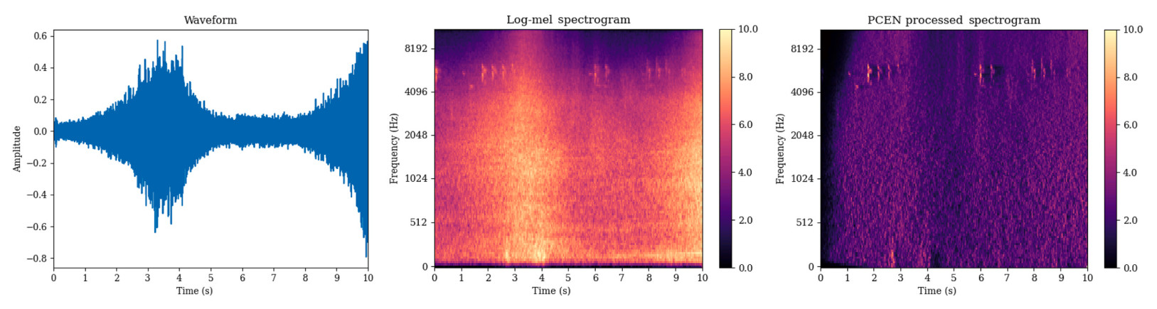
The specifics of PCEN processing are as follows: We utilize the STFT to convert the audio signal into the time-frequency domain and employ mel filters to capture the energy distribution across different frequency ranges. Notably, we design a mel frequency filter bank for the analysis of bird acoustic frequency characteristics, with a coverage range of 20 Hz to 10, 000 Hz to accommodate the frequency range of bird vocalizations. We set 128 mel filters to maintain a fine capture of audio signal features while reducing computational complexity and storage space requirements.
Subsequently, we apply an infinite impulse response (IIR) filter to the mel spectrogram for smoothing, generating a smoothed version M(t, f) to capture the signal’s loudness contour and emphasize the relative changes of the signal with respect to the recent spectral history. AGC stabilizes the signal level across different amplitudes by controlling an adaptive gain factor α ∈ [0, 1] that scales the smoothed spectrogram. Finally, power-law compression is applied to the scaled spectrogram, controlled by parameters δ and r, to further normalize the signal’s dynamic range, resulting in the PCEN-processed spectrogram. The specific parameter settings are shown in Table 3. The calculation process is given by Eq. (1):
PCEN(t,f)=(E(t,f)(ϵ+M(t,f))α+δ)r−δr
(1)
Table
3.
PCEN calculation process parameter settings.
The parameter settings for PCEN were determined through extensive experimentation and previous studies on audio signal processing. For instance, the adaptive gain factor α was set to 0.98 to balance noise suppression and signal preservation, while δ and r were set to 2 and 0.3, respectively, to effectively normalize the dynamic range of the audio signal.
The preprocessing effects of PCEN are shown in Fig. 1, where the original waveform of the sound and the spectrograms before and after PCEN processing are compared, clearly demonstrating the effectiveness of PCEN in audio signal processing.
Figure
1.
Visual comparison of audio before and after PCEN processing.
After PCEN processing, we extract MFCC and FCM features from the enhanced signal. Since the spectrogram of the audio signal has a better dynamic range and stability after PCEN treatment, we directly apply the Discrete Cosine Transform (DCT) to the enhanced spectrogram to convert frequency domain information into the cepstral domain. In this process, we retained the first 20 DCT coefficients. This selection is within a reasonable range (Huang and Bao, 2019; Jung et al., 2021), enabling effective capture of the key features of the audio signal while facilitating subsequent feature fusion. The resulting feature representation is denoted as PCEN-MFCC.
This transformation helps to extract the structured information of the signal, especially the periodic and harmonic structures related to audio signals, while retaining the advantages of MFCC in terms of energy concentration and high computational efficiency. Overall, PCEN-MFCC can reflect the spectral structure, temporal changes, and auditory perception characteristics of audio signals like MFCC, while offering better dynamic range compression and noise robustness.
For the extraction of FCM features, since the PCEN treatment has effectively suppressed noise and enhanced the signal, we can directly extract the required frequency components from the enhanced spectrogram without the need for traditional frequency binning steps. In this way, the PCEN-FCM features we construct can directly calculate the correlation coefficients between every pair of frequency components over the entire time period from the enhanced spectrogram. The correlation coefficients are calculated using Pearson correlation coefficients, as shown in Eq. (2):
In this equation, ρij represents the Pearson correlation coefficient between the i-th row and the j-th row, with values ranging from −1 to 1. Specifically, a value of 1 indicates perfect positive correlation, −1 indicates perfect negative correlation, and 0 indicates no linear correlation. Xi and Xj are the frequency components of the i-th row and the j-th row at the k-th time frame, respectively. meani and meanj represent the mean values of the i-th row and the j-th row, respectively.
In the end, the feature set we constructed consists of two types of feature vectors, PCEN-MFCC and PCEN-FCM, with dimensions of (1, 20, 862) and (1, 128, 128), respectively. These include denoised time-frequency domain features and frequency domain correlation information. This provides the model with comprehensive audio features, enabling it to learn and recognize bird audio more accurately.
2.3
Dual-Feature Enhancement Fusion Model
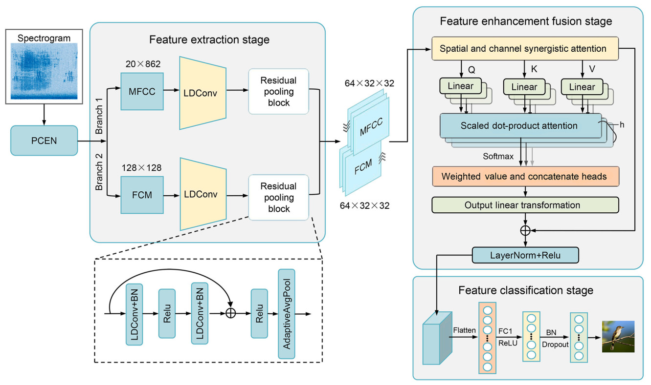
In this section, we introduce the proposed DFEFM, which includes three stages: deep feature extraction, feature fusion, and classification. FCM captures the correlations between frequencies, while MFCC extracts spectral features. The core of this model lies in its ability to integrate FCM and MFCC features to enhance detection performance. Figure 2 shows the entire process from feature extraction to classification.
In the feature extraction, we designed two parallel convolutional network branches to process MFCC and FCM inputs separately. This stage employs CNNs based on linear deformable convolution (LDConv) (Zhang et al., 2024), with the offset parameter of LDConv set to 4. LDConv is an improved convolutional operation that overcomes the limitations of traditional convolution, which has a fixed shape and a quadratic increase in the number of parameters, by introducing offset parameters and arbitrary sampling shapes. This allows the convolutional kernel to dynamically adapt to changes in the input signal, thereby capturing features more accurately. Additionally, the number of parameters grows linearly with the kernel size, enhancing computational efficiency and better aligning with hardware requirements. In our model, LDConv is applied to two parallel convolutional network branches. By dynamically adjusting the sampling shape of the convolutional kernel through offset parameters, it enhances the model’s adaptability and expressiveness for audio features. Moreover, its linear parameter growth characteristic alleviates the computational burden of the model. The specific network layer parameters are shown in Table 4.
Table
4.
The parameters for dual-branch CNN layers.
Subsequently, the feature maps are further processed by residual blocks composed of LDConv layers, batch normalization, and ReLU activation functions. This not only alleviates the vanishing gradient problem in deep networks but also enhances the training efficiency and stability of the model. Through the processing of multiple convolutional layers, the feature maps output by the two branches gradually approach each other in spatial dimensions. To achieve complete consistency in the size of the output features from both branches, the output of each branch is resized through an adaptive average pooling layer to align the feature structures. After alignment, the output features from both branches are concatenated on the channel dimension, forming a comprehensive feature map that integrates FCM and MFCC information, which is then sent to the feature enhancement fusion stage.
In the feature enhancement fusion stage, to enhance the expressiveness of the fused features, the model first introduces a SCSA module. This module enhances feature discriminability by focusing on key channels and spatial locations within feature maps through a shareable multi-semantic spatial attention mechanism and a progressive channel self-attention mechanism, thereby strengthening the model’s ability to recognize key information. The feature maps enhanced by SCSA are further processed using MHA mechanism. MHA maps the features into a higher-dimensional space through linear transformations of queries, keys, and values, and leverages parallel processing across multiple heads to integrate features at different scales while capturing long-range dependencies among features. Specifically, the computation of MHA primarily involves the following two dimensions.
1. Spatial Dimension: MHA operates over the height H and width W of the feature map, capturing relationships between different spatial locations within the feature map. This approach enables the model to simultaneously capture both local and global spatial dependencies, thereby providing a more comprehensive understanding of the distribution and interactions of features.
2. Channel Dimension: Although the primary attention computation is focused on the spatial dimension, MHA can also indirectly capture relationships between different channels through its multi-head mechanism. Each attention head can focus on a distinct subset of features, thereby enhancing the model’s ability to capture multi-scale features and further improving the representational capacity of the features.
The output of MHA, after linear transformation by the output layer, is combined with the original input features, ensuring information integrity and preventing information loss in deep networks. During the feature classification stage, the feature maps are first flattened, and then the fully connected layers map the high-dimensional features to category labels through linear transformations and activation functions, completing the classification task.
3.
Results and discussion
3.1
Experiment setup
During the training process, the same experimental hardware and software, as well as hyperparameter settings, were employed. The hardware and software used in the experiments are detailed in Table 5. To prevent overfitting, we utilized the early stopping method, and the main training configurations of the model are presented in Table 6.
Table
5.
Server and edge computing platform configuration.
To assess the specific impact of different feature inputs on the performance of BAD models, a series of ablation experiments were conducted in this section. In these experiments, we selected the raw MFCC features as the baseline input and employed the Linear Deformable Residual Convolutional Model (LDRCM), an early branch of the DFEFM model, as the baseline model. To ensure the reliability and stability of the results, we conducted five independent experiments. Each experiment utilized the same dataset partitioning (training set, validation set, and test set), but with different initial weights and random seeds. We recorded the ACC and area under the curve (AUC) for each experiment to evaluate model performance and calculated the mean and standard deviation of these metrics. ACC reflects the proportion of correctly predicted samples by the model, while AUC measures the model’s ability to distinguish between different classes, especially being more reliable in the context of imbalanced data. Table 7 presents the mean ACC and AUC values of different features and feature combinations across three publicly available datasets, as well as the overall average results across these datasets, revealing their specific impacts on model performance. Specifically, the standard deviations of ACC for all feature combinations across the three datasets did not exceed ±0.48%, and the standard deviations of AUC did not exceed ±0.58%. These results indicate high stability and reproducibility of the model performance.
Table
7.
ACC and AUC results for different feature combinations (value: ACC|AUC).
Analyzing the data in Table 7, we can observe variations in the ACC and AUC values of the model across different datasets, primarily due to differences in recording environments, bird species, and audio quality. For instance, the BirdVox dataset generally has lower ACC compared to the other two datasets, which can be attributed to its more complex recording environment, encompassing more background noise and interfering sounds.
When using a single feature input, the average ACC of MFCC and FCM are 79.1% and 81.5%, respectively, with average AUC values of 0.717 and 0.753. Notably, FCM outperforms MFCC as a single feature input, regardless of whether it has been processed by PCEN technology. This difference is particularly pronounced in the BirdVox dataset, where the ACC with FCM as input is 4.1% and 7.4% higher than with MFCC before and after PCEN processing, respectively. This suggests that FCM can effectively capture the frequency differences between bird audio and environmental sounds, thereby assisting the recognition model in detecting the presence or absence of bird vocalizations within the audio. Moreover, its performance surpasses that of MFCC, a representative feature of the time-frequency domain, proving the potential application of FCM in the field of BAD, especially in distinguishing bird audio from environmental noise in noisy backgrounds.
After PCEN processing, the performance of both MFCC and FCM features has been enhanced. The average ACC of MFCC after PCEN processing has increased to 81.3%, with an average AUC value of 0.748; for FCM, the average ACC has risen to 85.0%, and the average AUC value has improved to 0.809. These results confirm the effectiveness of PCEN in enhancing the dynamic range and stability of audio signals, particularly in suppressing background noise and increasing the salience of target sounds in distant scenes.
When the dual-feature enhanced fusion model receives MFCC and FCM as dual-feature inputs, the model performance significantly improves, with an average ACC of 87.7% and an average AUC value of 0.929. This enhancement indicates that a single feature can provide a certain level of recognition capability, but its performance is limited and cannot fully capture the complexity of audio signals. Our designed DFEFM model can reasonably incorporate the information contained in both features, thereby more comprehensively capturing the characteristics of audio signals and enhancing the model’s ability to distinguish between bird audio and others in recordings. Ultimately, when using PCEN-processed MFCC and FCM for dual-feature fusion, the model’s ACC reaches 91.4%, and the AUC value reaches 0.963, which is the best performance among all configurations. This not only proves the effectiveness of PCEN processing and dual-feature fusion in improving the ACC of BAD but also demonstrates the robustness of our method across different datasets, which is of significant value for wild bird monitoring and ecological research.
3.2.2
Comparison experiments with existing methods
Given that the application of feature fusion techniques in BAD is not yet widespread, our comparative experiments primarily focus on research methods that target the DCASE2018 dataset as well as methods that have performed well in the field of sound recognition over the past two years.
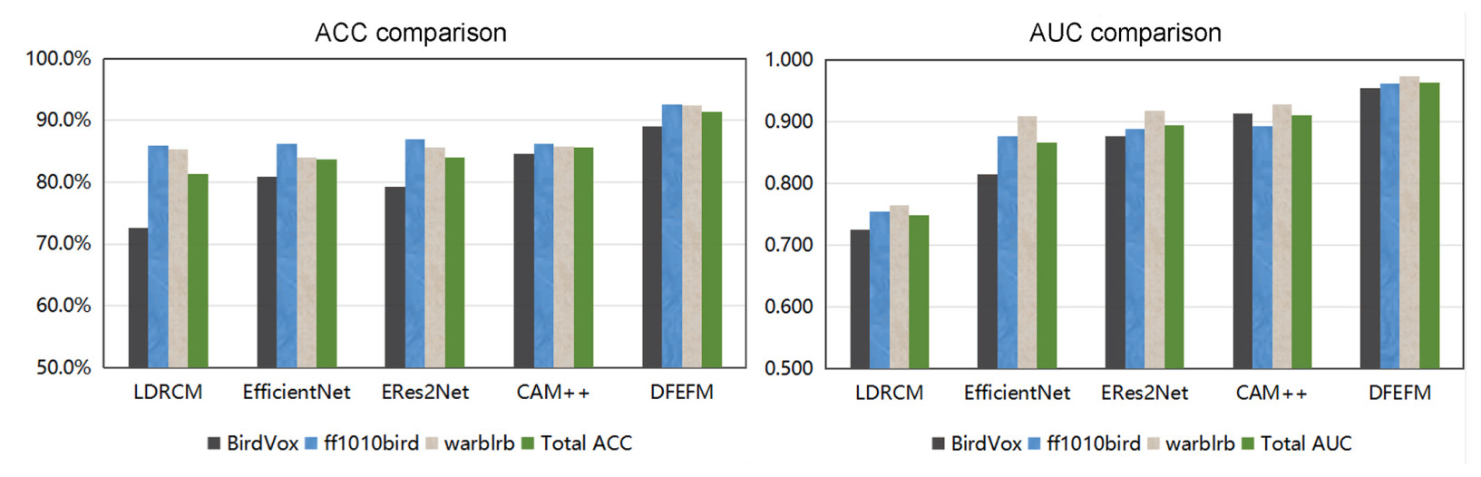
Anderson and Harte (2022) utilized the EfficientNet model (Tan and Le, 2019) to process spectrograms in their research approach, but this study did not provide detailed results across various datasets and relied mainly on ACC as a single evaluation metric. To provide a more comprehensive comparison, we selected the ERes2Net (Chen et al., 2023) and CAM++ (Wang et al., 2023) models, which have shown excellent performance in the field of sound recognition over the past two years, for comparative experiments. Originally designed to detect speaker characteristics from speech features, we adapted these models for BAD. Since these models are single-feature input models, we used MFCC features processed with PCEN as a unified input in our comparative experiments, with LDRCM serving as the baseline model. Figure 3 presents a visual comparison of the DFEFM against these sound recognition models in terms of ACC and AUC, while Table 8 provides the detailed results.
Figure
3.
Visual comparison of ACC and AUC results for different methods on the DCASE dataset.
Our experimental results show that EfficientNet improved the average ACC by 2.4% and the average AUC value by 0.119 compared to the baseline method, but its performance fluctuated significantly across different datasets. Particularly in complex audio environments with high background noise interference, such as BirdVox, the recognition ACC of EfficientNet dropped significantly, reflecting its shortcomings in noise resistance. This phenomenon may stem from EfficientNet not being specifically optimized for noise interference or its model architecture and feature extraction method not being entirely compatible with the features of bird vocalization.
ERes2Net, leveraging its local and global feature fusion techniques, improved the average ACC by 2.6% and the AUC value by 0.146 compared to the baseline method. However, ERes2Net’s performance across the three datasets was also not stable enough, which may be due to the limitations of its feature fusion techniques in capturing long-term sequential dependencies in bird audio or the loss of critical information when fusing multi-scale features.
In contrast, CAM++ demonstrated a relatively outstanding performance, particularly on the BirdVox dataset, which contains more background noise, achieving a significant improvement with an ACC of 84.6%. Overall, it improved the average ACC by 4.3% and the AUC value by 0.163 compared to the baseline, achieving the best results when using MFCC as a single feature input. This indicates that CAM++ can extract target sound features to some extent when dealing with complex audio signals, enhancing the model’s noise resistance capabilities.
Our method (DFEFM) innovatively utilizes two separate convolutional network branches to extract high-level representations of FCM and MFCC features at different scales, and significantly enhances the cross-modal information fusion capability of the merged feature maps through the cooperation of the SCSA module and MHA mechanisms. The average ACC and AUC metrics across the three datasets reached 91.4% and 0.963, respectively, which are significantly higher than those of EfficientNet, ERes2Net, and CAM++.
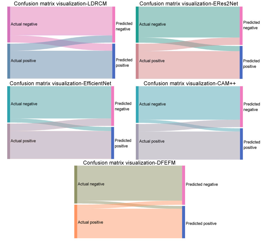
In addition to ACC and AUC values, we also used a Sankey diagram to visualize the comprehensive confusion matrices of the aforementioned models on the DCASE datasets (combining the results from the three public datasets), as shown in Fig. 4. Through the results of the confusion matrices, we can calculate the false negative rate (FNR) and false positive rate (FPR) of the models, as presented in Table 9. The experimental results indicate that DFEFM has the lowest FNR and FPR compared to the other four methods, further demonstrating the significant advantages of our approach in terms of ACC and reliability in detecting bird audio.
Figure
4.
Sankey diagram visualization of confusion matrices for five models.
3.2.3
Performance of DFEFM in real-world scenarios
To validate and assess the performance of DFEFM in real-world scenarios, we merged the three public datasets from the DCASE bird detection task and trained an initial model based on this combined dataset. Subsequently, we fine-tuned the model on the datasets from three different sites in Beijing (D1, D2, and D3). During the fine-tuning process, we froze the network layers before the MHA fusion module, a strategy aimed at preserving the model’s learned general feature representations from the DCASE2018 datasets while allowing the model to learn environment-specific features on the new datasets.
To further evaluate the generalization capability of the model and verify whether there is overfitting, we performed 3-fold cross-validation on our self-built datasets. The specific steps are as follows: each dataset was divided into three subsets. In each iteration, two subsets were used for training, and the remaining subset was used for validation. This process was repeated three times to ensure that each subset had the opportunity to serve as the validation set. Through cross-validation, we can better assess the model’s performance across different subsets, thereby evaluating its generalization ability. The results of the cross-validation are shown in Table 10.
Table
10.
Cross-validation results on self-built datasets (D1, D2, and D3).
The results indicate that on the D1 dataset, the model achieved an average ACC of 98.7%, an AUC value of 0.988, and an F1 score of 0.984, with a standard deviation not exceeding 0.65%. This demonstrates that the model performs very stably on this dataset without any apparent signs of overfitting. Although the ACC on the D2 dataset is slightly lower than the other two datasets, primarily due to frequent human activity and higher noise interference within the park, the standard deviation remains relatively small (1.07%), indicating that the model still has good generalization ability on this dataset. On the D3 dataset, the model achieved an average ACC of 97.5% with a standard deviation of 0.92%, further confirming the stability and generalization ability of the model across different datasets.
3.2.4
Performance of DFEFM on edge platforms
Considering that the detection model will be used on PAM devices, we further tested the performance of DFEFM and other comparative models on the NVIDIA Jetson Nano. We randomly selected 500 10-s bird vocalization segments from the DCASE2018 dataset for model inference testing, with results shown in Table 11.
Table
11.
Performance testing results on edge platforms.
According to the test results, LDRCM, as an early branch of DFEFM, demonstrated the shortest inference time (0.327 s), indicating our focus on computational efficiency during the design process. However, LDRCM’s ACC (79.13%) remains the lowest among all models.
EfficientNet and ERes2Net performed similarly in ACC, at 82.74% and 82.36% respectively, but showed significant differences in model parameter count and inference time. EfficientNet has with an inference time of 0.386 s, while ERes2Net has the longest inference time (0.838 s). CAM++’s ACC is 85.18%, once again confirming its superior recognition capabilities compared to EfficientNet and ERes2Net. However, its inference time is 0.683 s, which is relatively long. This may be due to the additional context-aware masking and multi-granularity pooling operations it needs to perform, which increase the computational burden. Our proposed DFEFM model has an inference time of 0.557 s. DFEFM’s inference speed is about twice as fast as ERes2Net’s and 48% faster than CAM++’s, only slightly behind EfficientNet. This is because DFEFM is designed with two independent convolutional network branches for deep feature extraction of dual features, enabling it to handle richer feature information. Although this may lead to a slight increase in runtime, DFEFM performs the best in ACC, reaching 89.48%.
In conclusion, considering the overall performance of model ACC and computational efficiency, DFEFM strikes an effective balance between these factors. This makes it highly suitable for real-time or near-real-time bird monitoring tasks, demonstrating significant practical value.
4.
Conclusion
Our study addresses the issue that the extraction of bird audio from PAM recording is susceptible to environmental noise interference, leading to a decline in BAD performance. We propose a novel BAD method based on the DFEFM for PAM devices. Firstly, we introduce PCEN to effectively suppress background noise and maintain the salience of bird audio. Then, we select the FCM and MFCC as feature inputs. DFEFM employs two parallel convolutional network branches to extract high-level features and learn information from both features, and integrates a SCSA mechanism with an MHA mechanism to enhance the model’s discrimination ability. The method proposed in this study surpasses the current best BAD methods on the DCASE2018 public dataset and also effectively detects bird audio on our self-built datasets from three different ecosystems in Beijing. Performance testing on NVIDIA Jetson Nano shows that the model demonstrates excellent processing efficiency. These results not only validate the effectiveness of our method but also prove its good generalization ability, making it suitable for deployment on edge monitoring devices. This method provides an efficient means of invalid audio filtering for bird vocalization collection on edge devices, helping to reduce the costs of edge storage and information transmission.
In the future, we plan to explore more types of audio feature fusion methods to enable the model to understand and interpret audio signals from different perspectives and more effectively detect bird audio. Enhancing the model’s stability in the face of complex environmental noise and improving its applicability in wild conditions will provide stronger technical support for bird conservation and ecological research.
This study involves no animal experiments; thus, no ethical approval is required.
Declaration of competing interest
The authors declare that they have no known competing financial interests or personal relationships that could have appeared to influence the work reported in this paper.
Acknowledgments
The authors are very grateful to the editors and anonymous reviewers for their guidance and useful suggestions. We are thankful to the DCASE2018 Bird Audio Detection Task Challenge for providing us with a substantial amount of open-source audio data.
Abdul, Z.K., Al-Talabani, A.K., 2022. Mel frequency cepstral coefficient and its applications: a review. IEEE Access 10, 122136–122158.
Anderson, M., Harte, N., 2022. Learnable acoustic frontends in bird activity detection. arXiv Preprint 2210.00889.
Apol, C.A., Valentine, E.C., Proppe, D.S., 2020. Ambient noise decreases detectability of songbird vocalizations in passive acoustic recordings in a consistent pattern across species, frequency, and analysis method. Bioacoustics 29, 322–336.
Berger, F., Freillinger, W., Primus, P., Reisinger, W., 2018. Bird audio detection-DCASE 2018. .
Chalmers, C., Fergus, P., Wich, S., Longmore, S., 2021. In: Modelling animal biodiversity using acoustic monitoring and deep learning. IEEE, Shenzhen, China, pp. 1–7.
Chen, Y., Zheng, S., Wang, H., Cheng, L., Chen, Q., Qi, J., 2023. An enhanced res2net with local and global feature fusion for speaker verification. arXiv Preprint 2305.12838.
Copiaco, A., Ritz, C., Abdulaziz, N., Fasciani, S., 2021. A study of features and deep neural network architectures and hyper-parameters for domestic audio classification. Appl. Sci. 11, 4880.
Frommolt, K.-H., 2017. Information obtained from long-term acoustic recordings: applying bioacoustic techniques for monitoring wetland birds during breeding season. J. Ornithol. 158, 659–668.
Haselhoff, T., Braun, T., Fiebig, A., Hornberg, J., Lawrence, B.T., Marwan, N., et al., 2023. Complex networks for analyzing the urban acoustic environment. Ecol. Inform. 78, 102326.
Hu, S., Chu, Y., Tang, L., Zhou, G., Chen, A., Sun, Y., 2023. A lightweight multi-sensory field-based dual-feature fusion residual network for bird song recognition. Appl. Soft Comput. 146, 110678.
Huang, A., Bao, P., 2019. Human vocal sentiment analysis. arXiv Preprint 1905.08632.
Jedrusiak, M.D., Harweg, T., Haselhoff, T., Lawrence, B.T., Moebus, S., Weichert, F., 2024. Towards an interdisciplinary formalization of soundscapes. J. Acoust. Soc. Am. 155, 2549–2560.
Jung, S.-Y., Liao, C.-H., Wu, Y.-S., Yuan, S.-M., Sun, C.-T., 2021. Efficiently classifying lung sounds through depthwise separable CNN models with fused STFT and MFCC features. Diagnostics 11, 732.
Lasseck, M., 2018. Acoustic bird detection with deep convolutional neural networks. In:
Detection and Classification of Acoustic Scenes and Events 2018, pp. 143–147.
Mitrović, D., Zeppelzauer, M., Breiteneder, C., 2010. Features for content-based audio retrieval. Adv. Comput. 78, 71–150.
Nichols, S.M., Bradley, D.L., 2019. Use of noise correlation matrices to interpret ocean ambient noise. J. Acoust. Soc. Am. 145, 2337–2349.
Pellegrini, T., 2017. Densely connected CNNs for bird audio detection. In: 2017 25th
European Signal Processing Conference (EUSIPCO). IEEE, pp. 1734–1738.
Ruff, Z.J., Lesmeister, D.B., Duchac, L.S., Padmaraju, B.K., Sullivan, C.M., 2020. Automated identification of avian vocalizations with deep convolutional neural networks. Remote Sens. Ecol. Conserv. 6, 79–92.
Segura-Garcia, J., Sturley, S., Arevalillo-Herraez, M., Alcaraz-Calero, J.M., Felici-Castell, S., Navarro-Camba, E.A., 2024. 5G AI-IoT system for bird species monitoring and song classification. Sensors 24, 3687.
Si, Y., Xu, H., Zhu, X., Zhang, W., Dong, Y., Chen, Y., et al., 2024. SCSA: exploring the synergistic effects between spatial and channel attention. arXiv Preprint 2407.05128.
Stowell, D., Wood, M.D., Pamuła, H., Stylianou, Y., Glotin, H., 2019. Automatic acoustic detection of birds through deep learning: the first bird audio detection challenge. Methods Ecol. Evol. 10, 368–380.
Symes, L.B., Kittelberger, K.D., Stone, S.M., Holmes, R.T., Jones, J.S., Castaneda Ruvalcaba, I.P., et al., 2022. Analytical approaches for evaluating passive acoustic monitoring data: a case study of avian vocalizations. Ecol. Evol. 12, e8797.
Tan, M., Le, Q., 2019. EfficientNet: rethinking model scaling for convolutional neural
networks. In: International Conference on Machine Learning. PMLR, pp. 6105–6114.
Verma, R., Kumar, S., 2024. AVIEAR: an IoT-based low power solution for acoustic monitoring of avian species. IEEE Sens. J. 24, 42088–42102.
Wang, H., Zheng, S., Chen, Y., Cheng, L., Chen, Q., 2023. CAM++: a fast and efficient network for speaker verification using context-aware masking. arXiv Preprint 2303.00332.
Wang, Y., Getreuer, P., Hughes, T., Lyon, R.F., Saurous, R.A., 2017. Trainable frontend for robust and far-field keyword spotting. In: 2017 IEEE International Conference on Acoustics, Speech and Signal Processing (ICASSP). IEEE, pp. 5670–5674.
Xie, J., Hu, K., Zhu, M., Yu, J., Zhu, Q., 2019. Investigation of different CNN-based models for improved bird sound classification. IEEE Access 7, 175353–175361.
Xie, J., Zhong, Y., Zhang, J., Liu, S., Ding, C., Triantafyllopoulos, A., 2023. A review of automatic recognition technology for bird vocalizations in the deep learning era. Ecol. Inform. 73, 101927.
Zeghidour, N., Synnaeve, G., Teboul, O., Quitry, F.D.C., Tagliasacchi, M., 2021. LEAF: a learnable frontend for audio classification. arXiv Preprint 2101.08596.
Zeghidour, N., Usunier, N., Kokkinos, I., Schaiz, T., Synnaeve, G., Dupoux, E., 2018. Learning filterbanks from raw speech for phone recognition. In: 2018 IEEE International Conference on Acoustics, Speech and Signal Processing (ICASSP). IEEE, pp. 5509–5513.
Zhang, X., Song, Y., Song, T., Yang, D., Ye, Y., Zhou, J., et al., 2024. LDConv: linear deformable convolution for improving convolutional neural networks. Image Vis Comput. 149, 105190.

 DownLoad:


 Email Alerts
 RSS Feeds